Getting Started with Binary Data Analysis: The Role of Entropy

Throughout this blog post series, we’ll explore the key techniques and methodologies used to understand and analyze raw binary data. Whether you’re working in cybersecurity, malware analysis, or reverse engineering, binary data analysis is an essential skill, without the right tools and approaches, it can be nearly impossible to interpret.

In this first post we’ll focus on entropy analysis, which introduces the broader world of binary data analysis. Entropy measures the randomness or unpredictability within a data set, and is a crucial tool for determining the structure of binary files and identifying compressed, encrypted, and random data within a file. This is especially important in fields like malware analysis, where understanding the nature of a file’s structure can reveal hidden threats or obfuscation techniques.

Generally speaking, areas of low entropy in a file could indicate repeated or predictable patterns, such as paddings, plaintext or uncompressed data. In contrast, areas of high entropy are often associated with encryption or compressed data, which could suggest hidden content or the use of obfuscation techniques.

As we continue through this series, we’ll cover more advanced topics in binary analysis. Each post will build on the previous one, offering insights and techniques that you can apply in real-world security scenarios.

So, let’s dive into entropy analysis and understanding why this foundational concept is the first step in uncovering the mysteries hidden within binary data.

Introduction to Binary Data Analysis: Understanding Entropy

Shannon entropy in few words

In the security field, entropy analysis is mostly used to detect packed and/or encrypted regions in a blob of data. This is usually done by the following Shannon entropy formula:

\[E = -\sum_{i} p(x_i)*log_2(x_i)\]

Where p(x_i) is the probability of appearance of the element x_i.

We will not deep dive into the mathematical aspect of Shannon’s formula in this blog post as there are many resources on the internet around the topic. However, for this article, we will re-use the following definition:

“At a conceptual level, Shannon’s Entropy is simply the “amount of information” in a variable. More mundanely, that translates to the amount of storage (e.g. number of bits) required to store the variable.”

To clarify the idea of a variable and its size, let us take a simple example of tossing a coin which yields one of two possible outcomes. A 1-bit variable could represent the raw data of the outcome, for example, the value 0 could represent a heads outcome and the value 1 could represent a tails outcome.

In the context of security work, a high entropy value typically means that the data is either packed or encrypted, which makes sense since we need more storage bits for our variable.

Entropy graph: A matter of offset and block size

In this section, we will perform an entropy analysis on a few firmware samples using Binwalk, a firmware reverse engineering tool.

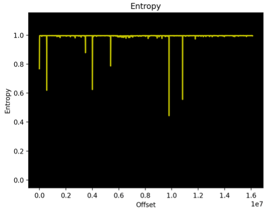
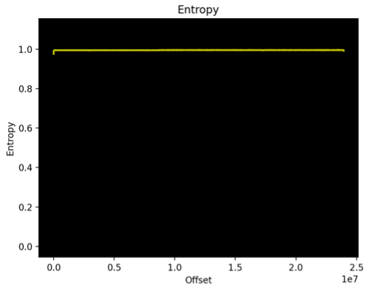
Figures 1 & 2 show an example of entropy graphs generated by the execution of Binwalk entropy analysis on two distinct firmware.


Figure 1. Entropy analysis for a NAS firmware RE_LAB % binwalk -E NAS_firmware.bin	Figure 2. Entropy analysis for a solar inverter firmware RE_LAB % binwalk -E INV_firmware.bin

We can see that there are a few entropy-falling edges in Figure 1 that do not appear in Figure 2. The actual offset in the “x-axis” reflects the position inside the firmware file itself. Those falling edges represent low entropy locations where we can find things like repeated bytes, patterns, “smaller” character space, etc.

But before taking any conclusions from the previous graphs, let us take a quick look at how an entropy graph is generated from a file.

If you look back at Equation 1 you will see that Shannon’s formula should generate a single value that defines the entropy of a blob of data. So how is the graph generated?

To generate an entropy graph, we need to split the file into blocks. We then calculate the entropy of each block, and plot the results. The x offset represents the block number, and the y value represents the block’s entropy.

Now a good question is: How is a block length defined?

Well, to illustrate this let us look at how Binwalk defines the block size. If you look at Binwalk source code, you will notice that if no block size is provided the block size will be derived from the file size and a constant defining the number of datapoints.

The following figures are taken from Binwalk source code:

    FILE_FORMAT = 'png'

    COLORS = ['g', 'r', 'c', 'm', 'y']

    DEFAULT_BLOCK_SIZE = 1024
    DEFAULT_DATA_POINTS = 2048

    DEFAULT_TRIGGER_HIGH = .95
    DEFAULT_TRIGGER_LOW = .85

    TITLE = "Entropy"

Entropy default datapoints and block size

            block_size = fp.size / self.DEFAULT_DATA_POINTS
            # Round up to the nearest DEFAULT_BLOCK_SIZE (1024)
            block_size = int(block_size + ((self.DEFAULT_BLOCK_SIZE - block_size) % self.DEFAULT_BLOCK_SIZE))
        else:
            block_size = self.block_size

        # Make sure block size is greater than 0
        if block_size <= 0:
            block_size = self.DEFAULT_BLOCK_SIZE

        binwalk.core.common.debug("Entropy block size (%d data points): %d" %
                                  (self.DEFAULT_DATA_POINTS, block_size))

Block size calculation

So, the block size (if not provided with -K argument) depends on the file size to generate those 2048 datapoints.

Why is the block size important?

The bigger the block size the more chances we will miss small low entropy chunks within it. Imagine we use a block size of 2048 bytes from which a chunk of 1920 bytes has high entropy and the remaining 128 have low entropy. The overall entropy of the block will remain high due to the negligible impact of the entropy of the 128 bytes.

Table 1 illustrates the previous example. We can see that the combination of the two files does not impact the high entropy of the block.

File name	Size (Bytes)	Description	Entropy
high_ent.bin	1920	Contains random data from /dev/random	0.988281
low_ent.bin	128	Contains ‘A’*128	0.008186
mixed_ent.bin	2048	Concatenation of the high and low files	0.966235

Table 1. Entropy analysis example

This minimal change in entropy would go unnoticed in an entropy graph with 2k points. Thus, we will miss the falling entropy edges in the graph.

Figures 1 & 2 are real-life examples of the problem. The size of the Solar Inverter firmware (Figure 2) is around 1.5 times larger than the NAS firmware. This results in Binwalk using a block size of 12k for the Solar Inverter compared to 8K for the NAS firmware.

So, one of the important things to keep in mind is to check the file size, use an appropriate block size, and pass it with -K argument otherwise it is possible to miss important zones in the firmware.

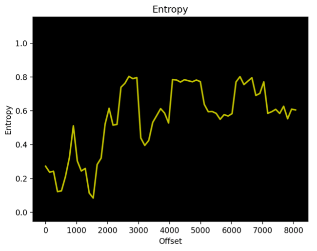
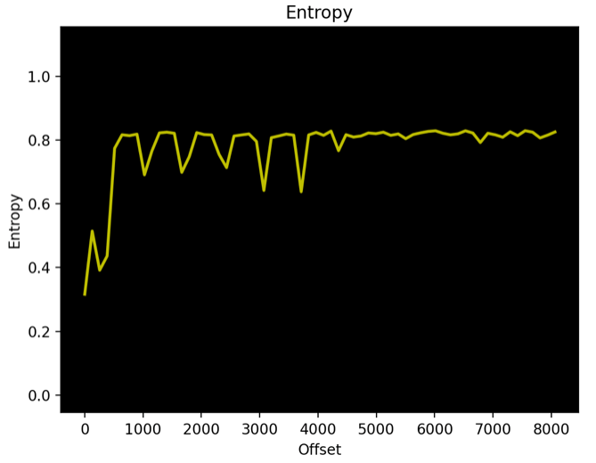
Figures 3 & 4 show the same analysis on the first 8k bytes (using -l parameter) using a block size of 128 bytes where we can see a more representative graph on the file entropy.


Figure 3. Entropy analysis for a NAS firmware RE_LAB % binwalk -E NAS_firmware.bin -l 8192 -k 128	Figure 4. Entropy analysis for a solar inverter firmware RE_LAB % binwalk -E INV_firmware.bin -l 8192 -k 128

That said, it is not always obvious to select a block size and an offset to start the analysis (could be provided with -o argument for Binwalk). A significant block size could be misleading, and a too-large block size could lead to missing important data chunks. On the other hand, a starting offset change could also impact the entropy of the blocks, as the calculation window will slide from its original position.

Entropy analysis: The thing in between.

Now that we have discussed entropy analysis and we understand how to interpret an entropy value, a question comes up. How high is “high entropy” and how low is “low entropy”?

Well, someone could say “Since we are talking about a probability distribution, a high entropy is 1 (or 8 if we talk about bits) and the lowest value is 0”. This is a correct statement but let us introduce the concept of high and low boundaries depending on the context.

If we think about several types of data (code, English text, assembly opcodes, encoded data, TLS certificates, etc.), they are each bound to their own specific syntax and format. For example, x86/64 assembly code is a formal language specified by a finite set of opcodes and rules. Sometimes data is even limited to a restricted set of characters (think English language or base 64 as examples).

If we understand the syntax of the data type for which we’re measuring entropy, we can bound low entropy and high entropy for that data type; the lower bound is primarily a function of redundancy, which reduces the entropy of that data to a specific lowest limit.

Use Case: English text

Let us take an example of detecting English text within a file. Shannon tackled this problem in diverse ways and published a nice paper titled “Prediction and Entropy of Printed English” which I would invite you to read if you are interested in the topic.

We know that the English language consists of 26 letters. For the sake of simplicity, we will not take the N-gram approach, but we can approximate the average entropy of a typical English text based on the frequencies of the alphabet letters in the English language, as shown in Figure 5.

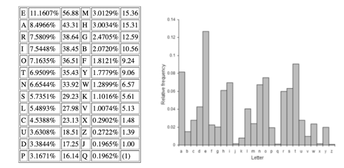
Figure 5. Frequency of letters in English text (source)

Since we have the probabilities of the appearance of each letter, we can calculate the average entropy of a typical English text.

probability=[11.1607,8.4966,7.5809,7.5448,7.1635,6.9509,6.6544,5.7351,5.4893,4.5388,3.6308,3.3844,3.1671,3.0129,3.0034,2.4705,2.0720,1.8121,1.7779,1.2899,1.1016,1.0074,0.2902,0.2722,0.1965,0.1962]
eng_entropy=0
for p in probability:
    eng_entropy -= p/100 * math.log(p/100, 2)
eng_entropy

4.246830567762619

Now we have our average mark of English text entropy which is around 4.2468. But what about the upper and Lower bound? From an intuitive reasoning we can guess the upper and lower bound values as follows:

The upper bound of an English text entropy could not exceed the entropy of a sentence of 26 letters containing one occurrence of each letter (Remember that redundancy leads to lower entropy) without any English language constraint. By applying the formula, we can deduce that an English text would never exceed an entropy of 4.70.
Getting a lower bound is a bit tricky as the smallest word in the English language contains one single letter which is “a” leading to an entropy of 0. But since we want a more realistic lower bound as a reference, we calculated the entropy of different random English texts of 128 characters, and the lowest entropy we hit was around 4.05.

Again, as a simple illustration, we found that a typical English text entropy may reside between 4.05 and 4.70 with an average approximated reference value of 4.2468 So, if we spot an entropy of a block within those values and close to our average reference there are big chances that it contains an English text.

Use Case: executable code regions

Similar to the estimation of English text entropy, we can estimate the upper and lower bound values and the average entropy value of a specific type of data if we know the rules to be applied and/or character sets to be used.

As another example, I would point the reader to the paper “Codescanner: Detecting (Hidden) x86/x64 Code in Arbitrary Files” where the researcher uses Shannon entropy analysis to classify blocks in a binary file, spotting possible executable code regions.

Let us put this into practice.

In this example, we will perform a quick entropy analysis on a solar solution communication interface firmware. The entropy graph in Figure 6 is generated by Binwalk against the firmware file.

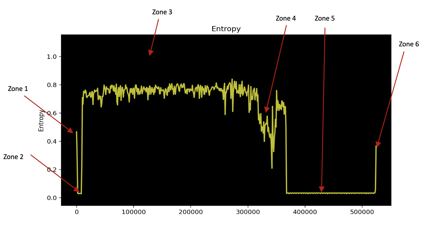
Figure 6. Entropy graph generated with binwalk

First, let us calculate the block size that is being used by Binwalk. As per Binwalk source code the block size is calculated by rounding the result of the division of file size by the number of desired datapoints (2048) to the nearest default block size (1024).

\[block\_size = \frac {file\_size}{2048} = \frac {524496}{2048}=256\]

Since 256 < 1024, Binwalk will round the block size to 1024.

Let us start the analysis with the default block size (1024) and see where it can lead us. We can clearly spot around 6 different zones.

Let us start looking at the first zone. This part is visible at the beginning of the picture where the entropy is approximately 0.45.

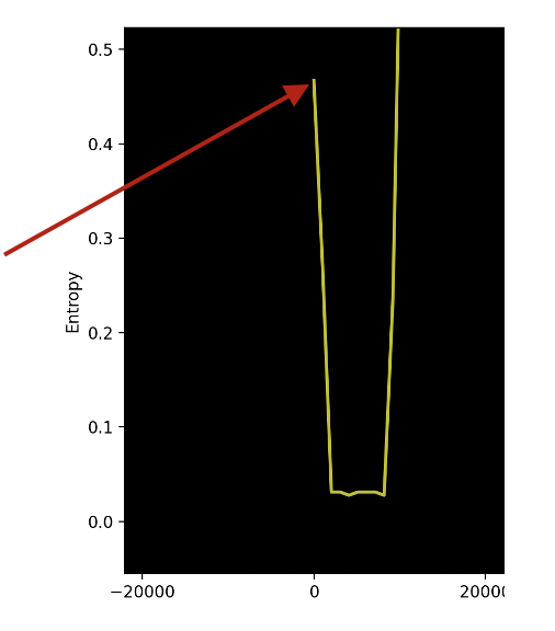
Figure 7. First zone in entropy graph

As per our discussion previously we can guess that the zone contains either:

Some strings: We saw earlier the statistics for the English text. However, since we are dealing with a binary file, we can guess that we are no longer bound to English text character frequency, but we are still in the spectrum of printable characters. We also may have punctuation and numbers that could raise a little bit the entropy above 0.45
A structure: We can also guess that the section is limited to a specific set of character set (Think English language entropy relying on 26 characters) which makes it a good candidate to be a kind of structure with repeated patterns but with a pretty wide range of character spectrum. So, it may contain addresses and offsets to some specific file locations.
A mix of strings and random data: This is what makes the entropy go a little bit above the 0.45 range
A high entropy part of compressed data mixed with a part of a low entropy zone with space or repeated bytes. This may explain why the entropy is around 0.45

We can see that we started with different options which will not help us.

What catches the eye is the next zone. It is a zone that comes right after it with a lower entropy. Figure 8 shows a zoomed-in view.

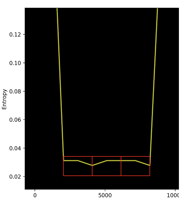
Figure 8. Zone 2 zoomed in

As per experience, we can see it looks to be presenting a kind of pattern (See red boxes in Figure 8). As per the first view of the two first zones, we can try to lower the block size to 128 bytes and generate the graph again.

Figure 9 shows a zoomed view of zones 1 and 2 using a block size of 128 bytes.

Figure 9. Zone 1 and 2 with a block size of 128 bytes (binwalk -K 128)

We can see that there is a pattern emerging. There is a stable entropy line that appears to be around 0.02x with two falling edges to an entropy of 0 in this zone. This makes us think about two scenarios:

Scenario 1:

There is a block with a specific structure using 3 to 4 different bytes. This is why the block has a very low entropy around 0.02x
There is a second block that is composed of one single byte repeated which explains the entropy value of 0.
This first block is repeated a few times before the second block begins
The first block size is a multiple of 128 while the second one is 128 bytes. This is deduced from the second block represented by a single drop point of entropy 0.

*Important note*: When we talk about a repeated block, this does not mean that the block is repeated as it is exactly. Remember that the entropy formula does not take into consideration the value of the byte itself. What it means is that there might be difference between the 1st appearance of block 1 and its second one. That said, the number of different characters in that block remains the same. The first explanation that comes to mind is that there may be an incremented index within the block that changes only one byte each time it is repeated.

Scenario 2:

There is only one single block that is repeated many times.
The block has a specific structure using 3 to 4 different bytes. This is why the block has a very low entropy around 0.02x
The block size is a little bigger than 128 bytes. This is why we see an entropy of 0.02x then a drop to 0 appears. The explanation is when the entropy calculation window of 128 shifts enough it will end up aligned with the part filled with only one byte so it will lead to an entropy of 0.
There is a second block that is composed of one single byte repeated which explains the entropy value of 0.
The first block size is a multiple of 128 while the second one is 128 bytes. This is deduced from the second block represented by a single drop point of entropy 0.
Same important note as scenario 1 related to the incremented index

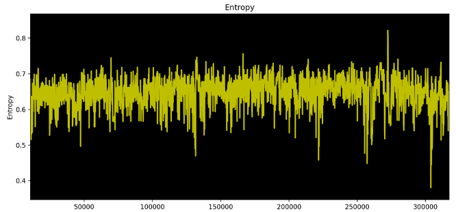
Figure 10. Zone 3 zoomed in

In Figure 10, we can see that zone 3 has a medium-high entropy ranging approximately between 0.6 and 0.7 with an average value of 0.6x. This could be in most cases a mix of random data, structure, and executable code.

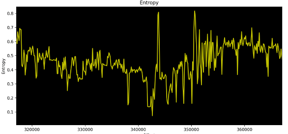Figure 11. Zone 4 zoomed in

Zone 4, as illustrated in Figure 11, shows a slight drop of entropy which is mostly around 0.4x and 0.5x. If you remember our explanation earlier, this zone could contain mostly text strings. Since we are dealing with binaries, we are not bound to our previous English text rules and thus sometimes going above the upper bound and sometimes going below the lower bound. Another reason for the entropy falls and rises could be due to existence of some structures, pointers and special characters that are used in binaries to store data and format text strings.

Zone 5 is another interesting one where we can use our previous knowledge from Zone 2. We can see a similar pattern that is repeated many times with falling edges to 0.

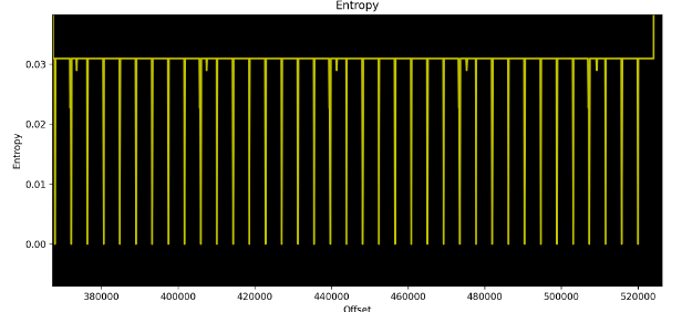
Figure 12. Zone 5 zoomed in

Since we can see a similar pattern between Zone 2 and Zone 5 we can take this exercise a step further. What we can do is analyze the graph and try to detect the exact size of the block structure.

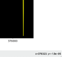
For this, we use scenario 2 from the analysis of Zone 2. We select two adjacent block numbers (offsets) where there is a falling edge to 0. Figures 13 and 14 show the values of 372095 and 376323.


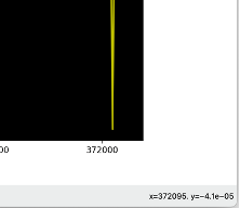Figure 13. First appearance of the falling edge	Figure 14. Second appearance of the falling edge

We know that our entropy block size is 128 bytes. If we divide the difference between the two offsets and subtract 1 we can know how many entropy blocks we calculated between the two points.

\[nb_{blocks} = \frac {376323-372095}{376323-372095} -1 = 32\]

We knew that we had to slide 32 blocks to rotate back to the initial state. This means that we have an excess of 4 bytes in our structure (128/32=4) making this rotation. So, the size of our structure appearing in Zone 2 and Zone 5 should be 132 bytes lengths where 4 bytes are most likely defining an index that is incremented at each repetition and 128 bytes of the structure itself are one single byte repeated.

This falls within our entropy estimation, as if we suppose that at Zone 2 the incremented index was represented by one single byte, we will have an entropy as follows:

128 bytes = 124 repeated byte + 1 byte incremented index + 3 bytes 0

We have 3 different bytes. One is repeated 124 times, one byte that changes after each block (the incremented index) and one byte (probably 0) repeated 3 times to pad the index to a double word.

By using the Shannon entropy formula, we can have:

\[ent_{zone2} = -\sum_{i} p(x_i)*log_2(x_i) = 0.282468457127818\]

This falls into what Binwalk graph shows for Zone 2

The same approach could be used to calculate the entropy of Zone 5. Here we know that our file is 512KB in length, if we divide that by our block size (128) we will get 4096 maximum blocks of 128 bytes. This means that only 2 bytes will be enough to hold its value. So, our 128-byte block will be as follows:

128 bytes = 124 repeated byte + 1 fixed bye + 1 incremented byte + 2 bytes of 0

Using the same Shannon entropy formula will get an entropy of 0.03093716553908933. This value makes sense and matches the entropy on Binwalk’s entropy graph for Zone 5.

Zone 6 is the last part of our file with an entropy of around 0.35. This is most likely another small structure with a bigger character space than the previous zone, but we will not deep dive into such a small zone from an entropy analysis approach.

In this example, we saw how we can apply our previous knowledge and perform a more in-depth entropy analysis on firmware and recognize some patterns and identify distinct zones to build up a first idea of the file structure.

Conclusion & takeaways

Entropy analysis is an effective way to identify the type of data blocks especially when dealing with unknown file structures. In this blog, we discussed different facets of Shannon entropy analysis that could be applied to various kinds of data such as firmware files, protocols, proprietary file formats, executable binaries, memory dumps etc. So, what are the key takeaways?

The bigger the character space (number of distinct characters) the higher the entropy tends to be. We need more bits of storage to represent all of our character space.
The more a specific character is repeated, the lower the entropy: We need a smaller number of bits in our variable to store the data.
When analyzing entropy graphs, ensure that you have used a proper block size otherwise the graph visualization could be biased, and you may be missing some important blocks.
The positions of the starting blocks could also lead to different results since a specific block of data could be split between two adjacent blocks, hence getting different entropy values.
If a data type has specific rules and/or relays on a specific set of character space, it is possible to calculate the upper bound, lower bound, and the average typical entropy value for. This will help identify the data block included in a file.
The order of appearance of the characters does not matter in the entropy calculation. The formula is based on the frequency of appearance of each character independently of its position so, keep in mind that the entropy of the string “AAAAC” is the same for “CAAAA”.
The entropy formula does not care about the byte values themselves. The formula takes only in consideration the number of distinct bytes (characters) and their distribution so keep in mind that the entropy of the string “AAAAB” is the same for “AAAAC”.

What else can I look at?

Rényi entropy: A generalization of the notion of entropy including Hartley entropy, Shannon entropy
Levenshtein distance: A measure for the difference between two string sequences.
Hamming distance: A measure for the difference between two string sequences.
Kullback–Leibler divergence: A measure of the difference between two probability distributions
Perplexity of a probability distribution: measures how well a probability distribution or a model could predict a sample.