Summary
Binary file analysis can be facilitated by segmenting the file into distinct regions and identifying unique patterns within each segment. As previously discussed in our article on Binary Data Analysis: The Role of Entropy, Shannon entropy can be leveraged to detect anomalous or high-entropy regions. This follow-up post delves into various programmatic techniques for systematically and reproducibly identifying these file segments, enabling a more comprehensive understanding of binary file structure and composition.
Time Series and Signal Analysis
A binary file is a one-dimensional array of bytes. By viewing these bytes as a time series (i.e., the byte index being the “time” axis), we can borrow a host of signal processing or time series analysis methods to aid in pattern detection.
Figure 1 shows 2048 bytes from a DVB receiver firmware plotted as a time series. On this plot:
- The X-axis corresponds to the byte offset in the file.
- The Y-axis corresponds to the byte value (0–255).
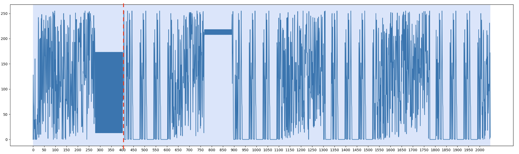
Figure 1. Plot of 2048 bytes of a firmware as time series
From this plot, we can visually identify two main sections (separated by a red dotted line):
- The first section is roughly offset 0 to offset 400.
- The second section spans from offset 400 to the end of the data.
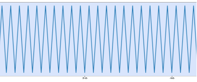
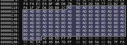
Within the first section (particularly around offset 280 to 400), a recognizable pattern emerges: several pairs of bytes where one is systematically higher than the next. Figure 2 zooms in on part of this region, while Figure 3 provides a corresponding view in a hex editor.
 |
 |
|---|---|
| Figure 2. Zoom in section 1 | Figure 3. Hex dump content |
In contrast, the second section appears to have a more consistent, repeating pattern characteristic of a structured region in the file. Figure 4 zooms in on part of this region, highlighting a pattern that repeats throughout the section:
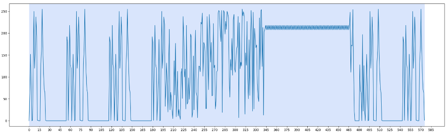
Figure 4. Section 2 structure zoom in
Notice that from approximately offset 190 to 470 (relative to the start of section 2), the structure is similar but includes additional data in one of its fields, resulting in a slightly “longer” repeated chunk.
Note: In many firmware images, you might see repeated headers or tables followed by variable-length fields that can appear visually similar but differ in length. Recognizing these repeated structures can reveal embedded code, configuration blocks, or cryptographic data segments.
Change Point Detection
A Survey of Methods for Time Series Change Point Detection defines change point detection as:
Change point detection (CPD) is the problem of finding abrupt changes in data when a property of the time series changes.
An Evaluation of Change Point Detection Algorithms also states:
…the presence of a change point indicates an abrupt and significant change in the data generating process.
Applying this idea to a sequence of bytes allows us to find offsets where the “distribution” of values changes significantly. This can help in identifying structurally distinct segments of a file, such as code vs. data, compressed vs. uncompressed regions, or even suspiciously encrypted sections.
ruptures Library Overview
We will use the Python library ruptures to illustrate how to automate some of these segmentations. ruptures offers six primary search methods for identifying change points:
| Method | Description | Models/Kernel | Prediction |
|---|---|---|---|
| Dynp | Finds optimal change points using dynamic programming. | l1, l2, rbf | n_bkps |
| Binseg | Binary segmentation. | l1, l2, rbf | n_bkps |
| BottomUp | Bottom-up segmentation. | l1, l2, rbf | n_bkps |
| Window | Window sliding method. | l1, l2, rbf | n_bkps |
| Pelt | Penalized change point detection. | l1, l2, rbf | pen |
| KernelCPD | Finds optimal change points (using dynamic programming or Pelt) for kernel-based cost functions. | linear, rbf, cosine | n_bkps, pen |
Table 1. ruptures change detection search methods
Two principal approaches can be gleaned from the “Prediction” column:
- Using a predefined number of breakpoints (
n_bkps). - Using a penalty-based approach (
pen), where the algorithm automatically determines the optimal number of segments.
Note: For quick analyses, specifying a small number of breakpoints like 1 or 2 can confirm large structural divisions. For advanced or highly granular segmentation (such as analyzing each section of firmware format), a higher number of breakpoints or a penalty-based approach can reveal more subtle transitions.
Examples with Dynp and Pelt (l1, l2, rbf Models)
Below is a minimal snippet for splitting our data into two sections using Dynp with the l1 model:
import numpy as np
import ruptures as rpt
import matplotlib.pyplot as plt

# Suppose 'data' is our list or numpy array containing byte values from the file:
signal = np.array(data)

# Choose the Dynp search method (dynamic programming) with model="l1".
algo = rpt.Dynp(model="l1").fit(signal)

# Ask for a single breakpoint, effectively dividing the data into 2 segments.
result = algo.predict(n_bkps=1)

# Display the segmentation:
rpt.display(signal, result, result, figsize=(20, 6))
print("Detected breakpoints:", result)
plt.show()
Similarly, for the Pelt method with a penalty approach:
algo_pelt = rpt.Pelt(model="l1").fit(signal)
result_pelt = algo_pelt.predict(pen=10)  # Example penalty value
print("Detected breakpoints (Pelt):", result_pelt)
 |
 |
 |
|---|---|---|
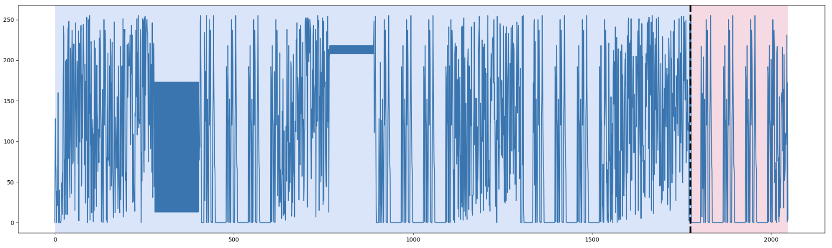
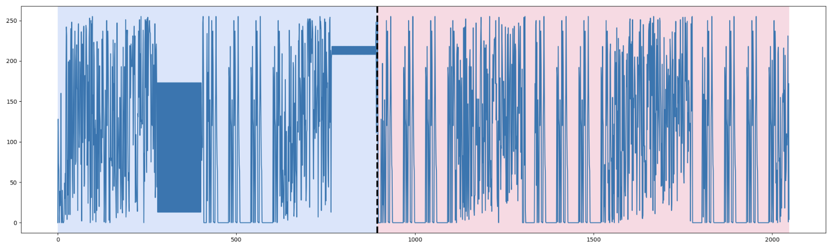
| Figure 5. Dynp with model l1 and n_bkps=1 | Figure 6. Dynp with model l2 and n_bkps=1 | Figure 7. Dynp with model rbf and n_bkps=1 |
Figures 5, 6, and 7 (in previous examples) show the results of using Dynp with the l1, l2, and rbf models respectively, each dividing the data into two segments (n_bkps=1). We see that l2 and rbf often come closest to matching the large-scale boundary we identified manually.
Increasing the Granularity
If we increase n_bkps to 9 (resulting in ten segments), we obtain a more granular breakdown. Many smaller repeating patterns become evident, which can be especially beneficial if we suspect multiple substructures or small embedded data blocks.
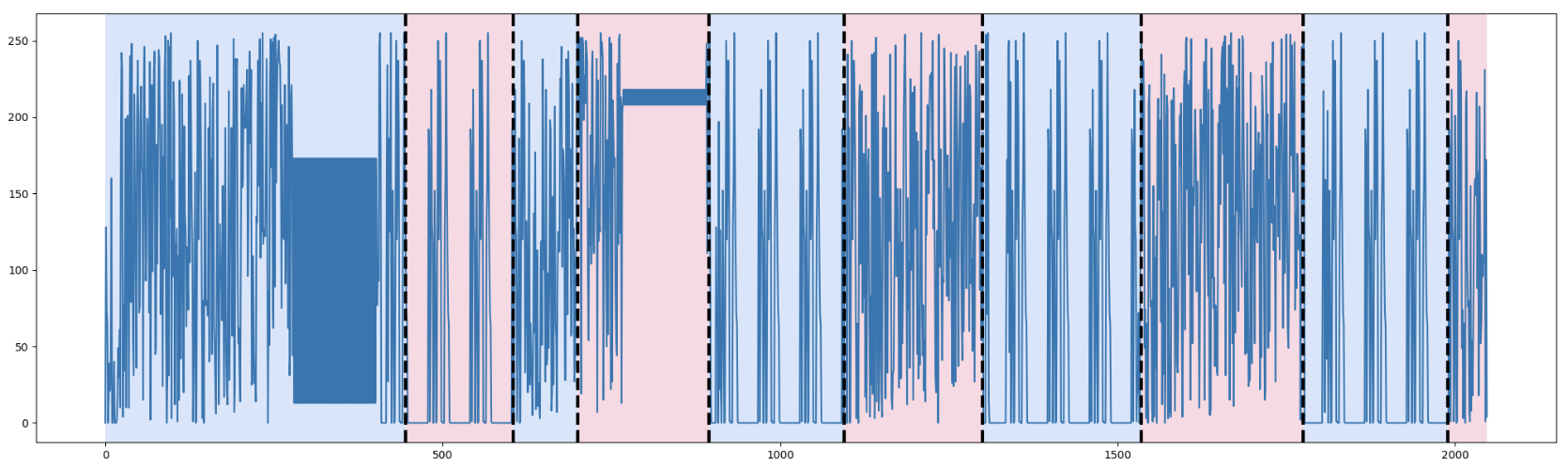 Figure 8. Dynp with model l1 and n_bkps=9
Note: In practice, you might adjust the penalty or the number of breakpoints based on domain knowledge. For example, if you suspect multiple repeated protocol headers or sections, a higher n_bkps might be warranted.
from ruptures.base import BaseCost
import math

def shannon_ent(data_block):
    # Basic Shannon entropy function
    from collections import Counter
    length = len(data_block)
    if length == 0:
        return 0.0
    counter_vals = Counter(data_block)
    entropy = 0.0
    for val in counter_vals.values():
        p = val / length
        entropy -= p * math.log2(p)
    return (entropy / 8.0)  # Optionally scale by 8, or any factor

class ShannonCost(BaseCost):
    model = ""
    min_size = 2

    def fit(self, signal):
        self.signal = signal
        return self

    def error(self, start, end):
        sub = self.signal[start:end]
        return (end - start) * shannon_ent(sub)
Adjusting Penalty and Breakpoints
In practice, you might adjust the penalty or the number of breakpoints based on domain knowledge. For example, if you suspect multiple repeated protocol headers or sections, a higher n_bkps might be warranted.
Getting Better Results: Using a Custom Cost Function
One of ruptures’ powerful features is the ability to define a custom cost function. In our previous blog post, we discussed how to use Shannon entropy to help identify compressed or highly random (possibly encrypted) regions. Normally, you might achieve this by chunking the file at fixed intervals and calculating entropy for each chunk. However, with a custom cost function, you can allow the algorithm itself to create segments where the entropy distribution varies.
To do so, we will rely on the fact that ruptures allows us to define a custom cost function. We will define our cost function based on the entropy of the segment.
The following Python code implements our ShannonCost class that returns a value based on the calculated Shannon entropy of the segment.
Shannon Entropy as a Cost
In the following snippet, we create a custom cost function class that multiplies the Shannon entropy of a segment by its length in bytes. This way, large segments with different entropy characteristics are more likely to form distinct segments.
from ruptures.base import BaseCost
import math
from collections import Counter

def shannon_ent(data_block):
    # Basic Shannon entropy function
    length = len(data_block)
    if length == 0:
        return 0.0
    counter_vals = Counter(data_block)
    entropy = 0.0
    for val in counter_vals.values():
        p = val / length
        entropy -= p * math.log2(p)
    return (entropy / 8.0)  # Optionally scale by 8, or any factor

class ShannonCost(BaseCost):
    model = ""
    min_size = 2

    def fit(self, signal):
        self.signal = signal
        return self

    def error(self, start, end):
        sub = self.signal[start:end]
        return (end - start) * shannon_ent(sub)
Example usage
algo = rpt.Dynp(custom_cost=ShannonCost()).fit(signal)
result = algo.predict(n_bkps=1)
Running the same code to split our data into 2 sections will result in Figure 9.
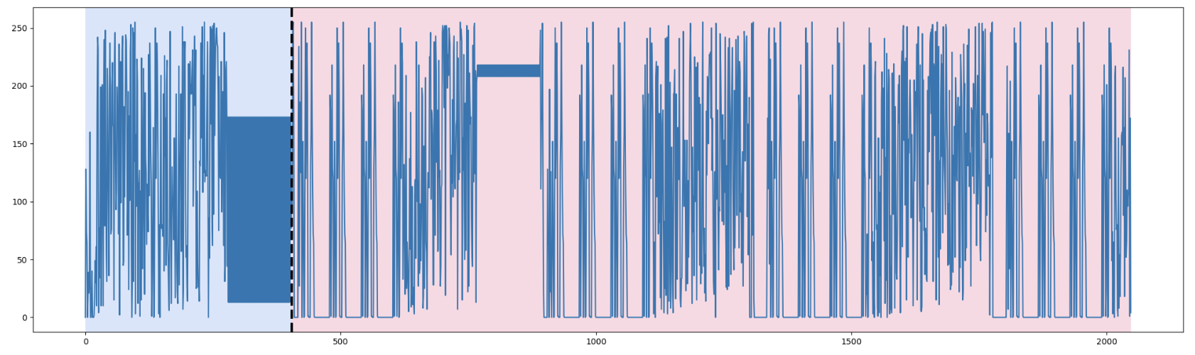 Figure 9. Dynp with custom cost function and n_bkps=1
When we run the above with n_bkps=1, we often see that the identified boundary closely matches the large-scale transition observed visually. If we again increase n_bkps to a larger number (say 7 or 10), we can detect multiple substructures based on significant entropy changes—this often performs better than, for example, the generic l1 model, when we specifically want to find transitions from lower-entropy to higher-entropy data.
We can also conduct another test with n_bkps=7 as we did previously and compare the results with the l1 model of Dynp.
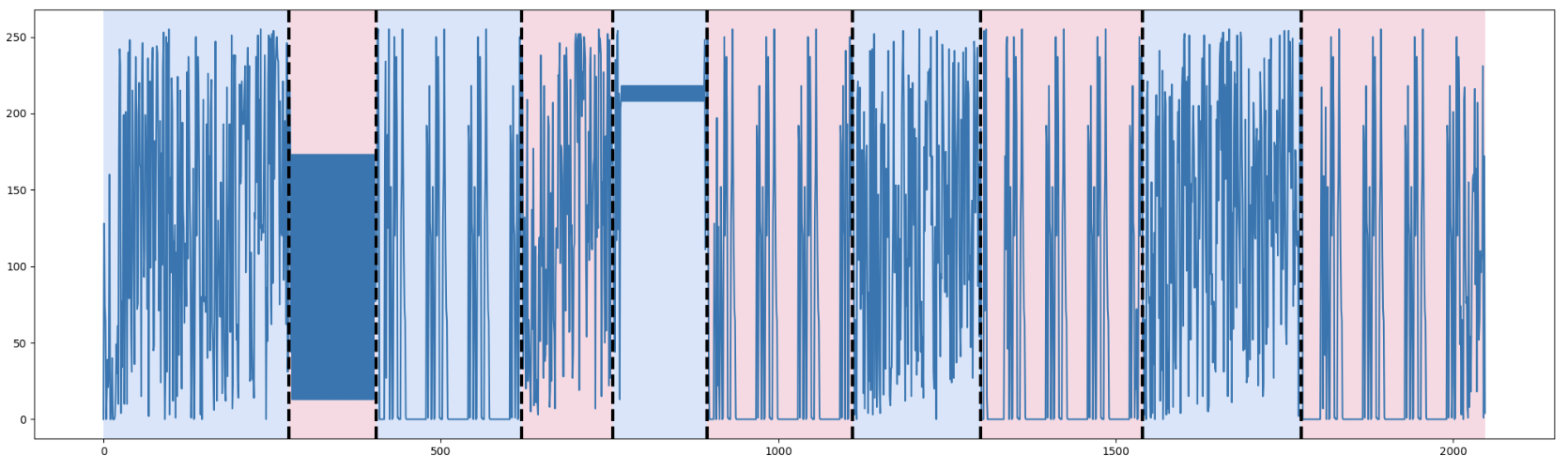 Figure 10. Dynp with custom cost function and n_bkps=10
If we compare the result of our custom cost function in Figure 10 to the one using model l1 in Figure 8, we can see that we achieved better results in detecting different patterns.
We can see, for example, that we detected the two patterns based on two repeated bytes (Block 2 and Block 5). We also were able to detect our repeated structure (Block 3, 6, 8, 10).
Note: In security research, segments with abnormally high entropy might signal encryption or compression. Conversely, extremely low-entropy segments could be zero-padded or contain repeated identical data (e.g., blank memory areas in firmware). Identifying these transitions is vital for subsequent forensics or reverse engineering steps.
To this point, the primary approach to segmentation relies on Shannon entropy and standard ruptures methods (Dynp, Pelt) without further optimization of the entropy function. This code demonstrates how to compute Shannon entropy in pure Python (often iterating over data in a Python loop). Although this works for small or single files, performance can degrade when handling large firmware images or repeated analyses. In real-world security research, the overhead becomes significant if you process thousands of blocks or large binaries.
Examining the below Shannon-igans.py, notice it defines an @njit function named optimized_shannon_ent which is used inside an OptimizedShannonCost class (derived from ruptures’ BaseCost). This change is crucial because “nopython” mode prevents Numba from falling back to Python objects, thereby producing a true machine code path for numeric operations.
Here’s how the optimized_shannon_ent function looks:
@njit
def optimized_shannon_entropy(data: np.ndarray) -> float:
    """Calculate Shannon entropy of the input data using Numba optimization."""
    counts = np.bincount(data)
    total = data.size
    nonzero_counts = counts[counts > 0]
    probabilities = nonzero_counts / total
    return -np.sum(probabilities * np.log2(probabilities))


class OptimizedShannonCost(BaseCost):
    """Custom cost function using optimized Shannon entropy."""
    model = "OptimizedShannon"
    min_size = 2

    def fit(self, signal):
        self.signal = signal
        return self

    def error(self, start, end):
        sub = self.signal[start:end]
        return (end - start) * optimized_shannon_entropy(sub)
How the optimized_shannon_ent Function Works
-
@njit compiles the function once, reusing the compiled version on subsequent calls. For Shannon entropy, this is particularly important if you’re scanning many blocks, e.g., in a sliding window or in repeated calls by ruptures.
-
Numba internally transforms the Python AST into LLVM IR (Intermediate Representation). This IR is then optimized and JIT-compiled to native code. Because the Shannon entropy formula is mostly array operations, it maps well to Numba’s numeric optimizations.
-
As a result, you typically see up to a 10× or more speed improvement for large data arrays, as confirmed by user reports in the Numba discussion forums and performance tips.
-
The difference in overhead is especially noticeable in repeated calls—the previous Shannon Python-based entropy calculations might re-compute frequencies in Python loops many times, whereas the Numba approach leverages faster memory access and reduced Python function call overhead.
In order to refine performance and optimization, you can tweak your chunk sizes or the cost function. Because the new entropy function is faster, you can try more fine-grained chunking or run more CPU-intensive analyses. This allows deeper exploration of your firmware’s structure.
In short, both script approaches rely on a purely Python-based Shannon entropy method. Both work, but the optimized Shannon entropy script is more efficient for large-scale or repeated analyses.
Researchers often choose a high-entropy binary from RANDOM.ORG’s Pregenerated File Archive, such as the December 2024 .bin entry, because it provides a large block of genuinely random data that drives the “Shannon-igans.py” script to its limits. Unlike a contrived or trivial test file, truly random bytes from RANDOM.ORG have a nearly uniform distribution across all possible values, which highlights the script’s performance and accuracy under “worst-case” entropy conditions.
Using a random.org binary thus stress-tests change-point detection, helping the researcher ensure the optimized Shannon entropy code is robust to noise and doesn’t produce excessive false positives. Moreover, because each byte is unpredictable, segments of random data can reveal how quickly or accurately the script pinpoints “boundaries” in data that truly exhibit maximum uncertainty. This is preferable to a simple, artificially generated file, which might be repetitive or only partially random, yielding fewer insights into the script’s real-world reliability. This example below uses the random.org binary from 2024-12-20.
One-Dimensional Heatmap of Firmware Bytes Showing Detected Change Points
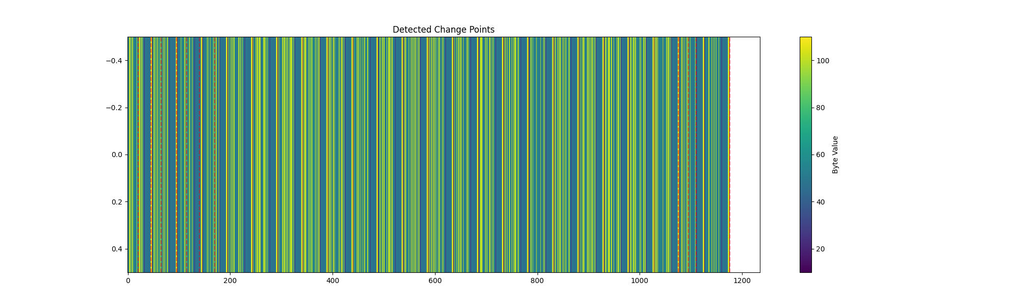 Figure 11. One-Dimensional Heatmap of Firmware Bytes Showing Detected Change Points
The red dashed vertical lines in Figure 11 are the change points (or “breakpoints”) that the script identifies as boundaries between distinct segments in the binary data. Specifically, after the script computes an optimized Shannon entropy–based cost (via OptimizedShannonCost) and calls ruptures’ Dynp method to predict breakpoints, those breakpoints get plotted with red vertical lines:
• The script’s detect_change_points method uses rpt.Dynp(custom_cost=OptimizedShannonCost()) to find change points.
• Once it obtains a list of those offsets (e.g., [120, 234, 480, …]), the visualize_change_points function draws each one as a red dashed line by calling plt.axvline(x=cp, color=’r’, linestyle=’–’).
Each red line corresponds to an offset where the algorithm decides there is a significant shift in the distribution of bytes, based on entropy measurements. This parallels the earlier examples, which describe how red dotted lines “delimit” different sections after performing a similar segmentation. Essentially, Figure 11 is a heatmap (or “barcode” style) visualization of the firmware data, overlaid with vertical red lines where the segmentation algorithm has identified structural boundaries.
ServiceNow Security Research released Shannon-igans, a tool designed to automate the enhanced segmentation and visualization of binary files, as showcased in Figure 11. This release, named shannon-igans, leverages optimized Shannon entropy calculations via Numba, change point detection with ruptures, and visualizations using Hilbert curves and UMAP, to identify distinct patterns and anomalies. The tool also generates a summary table with segment details, including entropy values and class labels, clustered using K-means.
Additional Insights from the Kudan Repository Code
The Kudan repository, Kudan, provides several utility functions (in a file named utils.py) tailored for binary analysis, such as:
- Computing byte-value distributions and Shannon entropy.
- Sliding window approaches for repeated pattern detection.
- Levenshtein-based distance checks on extracted strings or hex slices.
- Higher-level segmentation with algorithms like Pelt and Dynp (custom or built-in cost functions).
Below are some highlights that might be particularly useful:
repeated_pattern_stats: Detects repeated byte patterns of a given size, useful for discovering repeated protocol headers or repeated blocks.longestRepeatedSubstring: Identifies the longest repeating hex substring, which can reveal zero-padded areas or leftover debugging code.detect_outliers: Employs a multi-step approach (entropy, Levenshtein distance, TF-IDF-based clustering) to detect anomalies or malicious embeddings.
When to use the Levenshtein distance approach in a Security Research practice
Levenshtein distance is a way to measure how many single-character edits (insertions, deletions, or substitutions) are needed to transform one string into another. In the context of firmware or binary analysis, you can leverage this technique for several reasons:
Reason 1: Detecting Similar but Not Identical Strings
This involves identifying near-duplicate or minor variations of strings that could otherwise be overlooked. For example, when extracting strings or hex slices from a binary, some may appear very similar but differ in a few characters, such as variable names, obfuscated text, or partial encryption.
Reason 2: Spotting Anomalies or Suspicious Patterns
A Levenshtein distance check can help identify intentionally altered artifacts in malicious firmware. By quantifying “how different” an altered string is from a known benign string, you can prioritize further investigation into items that deviate from a known baseline.
Reason 3: Clustering or Grouping Related Segments
Levenshtein distance can be used to group strings or hex slices according to their similarity. If their distance to one another is small, they might represent different versions or minor tweaks of the same code region. This allows automated grouping and can highlight outliers.
Reason 4: Balancing Accuracy and Performance
Compared to other similarity measures, Levenshtein distance is relatively straightforward to implement and interpret. It can be combined with more advanced techniques to build a multi-layered approach for detecting anomalies in firmware or binary data.
In short, Levenshtein distance checks add an extra layer of detection for “near-similar strings,” boosting your ability to root out hidden or subtly modified code segments—especially when exact signature matches might miss small yet critical mutations.
Enhancing Firmware Analysis with TF-IDF
We’ve already seen how segmenting the binary via Shannon entropy can reveal structurally distinct chunks of data. However, once these segments are identified, we often extract meaningful substrings—configuration keys, code fragments, or error messages—and feed them into TF-IDF to quantify how unique or relevant each token is. When combined with clustering (e.g., k-Means) or outlier detection, TF-IDF reveals which segments contain highly distinct or anomalous textual data, thereby flagging areas of interest for deeper security forensics or reversing work.
As demonstrated in “utils.py,” the “detect_outliers” function employs a multi-step process that includes TF-IDF vectorization before clustering. After transforming strings into TF-IDF vectors, unusual strings are detected as outliers based on their centroid distance or distributional properties. This multi-step approach dovetails effectively with the entropy-based segmentation from “Shannon-igans.py,” creating a layered framework, as follows:
- Segment the firmware file by entropy changes.
- Extract or parse the strings from those segments.
- Finally, apply TF-IDF to measure the significance and rarity of tokens, enabling outlier detection on potentially suspicious code or data.
Through such TF-IDF-based filtering, analysts can prioritize investigations on firmware segments that exhibit not only high or low entropy but also anomalies at the text level, for example, repeated blocks with subtle textual modifications or embedded code fragments that contain unique function names. This layered methodology is particularly powerful when working with large firmware images and looking for a “needle in a haystack,” as TF-IDF reduces noise by spotlighting strings with distinctive token usage.
Note: Combining segmentation and search techniques can be powerful. After you identify abrupt changes in cost or entropy, you can investigate each segment in detail with known signatures, pattern matching, or advanced anomaly detection.
Source Code
All source code for this article, including the code snippets mentioned above, is in the Kudan repository. The repository also contains:
- Example scripts demonstrating how to load a firmware file as an array of bytes and run
ruptures. - Utilities (like
utils.py) for deeper exploration of repeated patterns, outliers, and segment-based analytics. - Visualization helpers for quick inline plots of segmentation results and entropy distributions.
The source code for Shannon-igans.py is here.
Key Takeaways
- Viewing a binary file as a signal or time series allows the application of robust change detection algorithms, revealing significant transitions in structure.
- The choice of cost function (
l1,l2,rbf, or a custom entropy-based approach) and segmentation strategy (n_bkpsvs. penalty-based) strongly influences the identified boundaries. - A custom cost function—such as one based on entropy—can be far more effective at revealing shifts between compressed/encrypted regions and plain data.
- Supplemental utilities (e.g., repeated pattern detectors, outlier detection using Levenshtein distance or TF-IDF clustering) add deeper layers of insight, making firmware and binary analysis more automated. (see https://github.com/aniketbote/Document-Clustering-TFIDF and https://github.com/roy-ht/editdistance for Levenshtein distance)
- Researchers often chain these steps:
- Segment the data with a general or custom cost function.
- Compute advanced statistics (patterns, outliers) within each segment.
- Investigate suspicious segments with disassembly or domain-specific heuristics.
-
Signal-based analysis: Treating binary files as signals or time series data enables the use of robust change detection algorithms, which can reveal significant structural transitions.
-
Cost function and segmentation strategy: The choice of cost function (e.g., l1, l2, rbf, or custom entropy-based) and segmentation approach (e.g., n_bkps vs. penalty-based) significantly impacts the identified boundaries.
-
Custom cost functions: Entropy-based cost functions can be particularly effective in detecting shifts between compressed/encrypted regions and plain data.
-
Supplemental utilities: Tools like repeated pattern detectors, outlier detection using Levenshtein distance or TF-IDF clustering, can add deeper layers of insight and automation to firmware and binary analysis.
-
Chaining analysis steps: Researchers often follow a workflow that involves:
- Segmenting data with a general or custom cost function
- Computing advanced statistics (e.g., patterns, outliers) within each segment
- Investigating suspicious segments using disassembly or domain-specific heuristics
By carefully tuning segmentation and analysis parameters, security researchers and forensic investigators can gain deeper insights into unknown binaries, a crucial skill in modern security research and investigations.